Autoselect Number of Lags for Augmented Dickey-Fuller Test
Testing a time series for a unit root is an important early step in a econometric model building workflow. Consider conducting the augmented Dickey-Fuller test for a unit root (null model) against an alternative model, whose structure is set by your specifications. Often, an appropriate structure for the alternative model is difficult to know at this point in a model building workflow. This example shows a method that automatically selects the number of lagged difference terms for the trend-stationary alternative model of an augmented Dickey-Fuller test. To determine which alternative model is best from a set of models that contain a varying number of lagged difference terms, the method uses Akaike information criterion (AIC).
Preprocess Data
Load the US macroeconomic data set named Data_USEconModel.mat.
load Data_USEconModelCompute the log of the GDP and include the result as a new variable called LogGDP in the data set.
DataTimeTable.LogGDP = log(DataTimeTable.GDP);
T = height(DataTimeTable);
Examine Data
Characterize the log GDP series by plotting it.
plot(DataTimeTable.Time,DataTimeTable.LogGDP)
xlabel("Year")
ylabel("Log USD Billions")
title("Log of GDP")
grid on
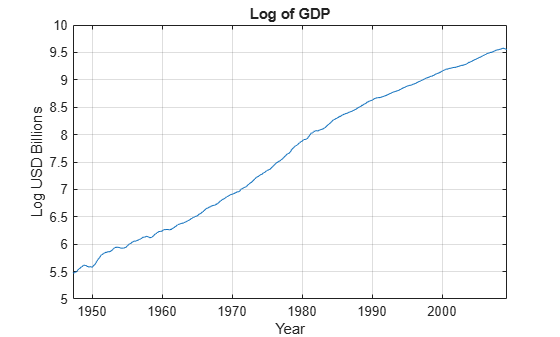
This series is clearly nonstationary. Because the log GDP series appears to have a linear, deterministic trend, the trend-stationary alternative model might hold.
Partition Data
To avoid data snooping, split the time series into two sets: a training set and a holdout set.
Training set — Determine the number of lags for the test by finding the best fitting model using the AIC.
Holdout set — Conduct the test using the optimized lag.
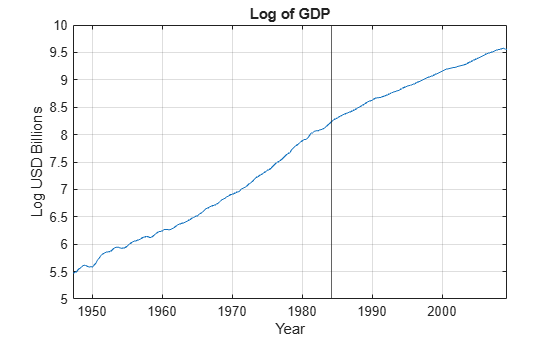
Split the data such that the training and test sets demonstrate a similar behavior and enough data exists to fit the alternative model. Use the slider to visualize the split.
TTrain =149; plot(DataTimeTable.Time,DataTimeTable.LogGDP) hold on xline(DataTimeTable.Time(TTrain)) xlabel("Year") ylabel("Log USD Billions") title("Log of GDP") grid on hold off
Create the training and holdout data sets.
trainingSample = DataTimeTable(1:TTrain,:);
testSample     = DataTimeTable((TTrain+1):end,:);
Find Optimal Number of Lagged Difference Terms
Using the training set, test for a unit root in the log GDP series using alternative models containing zero through four lagged difference terms. Return the regression statistics for each alternative model.
lags = 0:4;
[~,regstats] = adftest(trainingSample,DataVariable="LogGDP", ...
    Model="TS",Lags=lags);
regstats is a 5-by-1 structure array containing regression statistics from fitting the five alternative models required to run each test.
Extract the AIC values from the results table, and then plot them to visually determine the minimum. Extract the lag corresponding to the minimum AIC.
AIC = [regstats.AIC]';
plot(lags,AIC,"*-r")
xlabel("Number of Lagged Differences")
ylabel("AIC")
title("AIC for Models with Different Lagged Difference Terms")
grid on
hold on
[minAIC,minIdx] = min(AIC);
minLag = lags(minIdx)
minLag =
1
h = plot(minLag,minAIC,'bo',MarkerSize=15);
legend(h,"Minimum AIC")
hold off
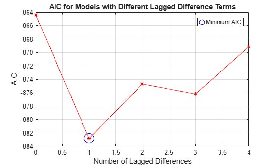
The lag associated with the minimum AIC during the training set is 1.
Conduct Augmented Dickey-Fuller Test
Perform an augmented Dickey-Fuller test for a unit root in the holdout set. Specify the optimal number of lags, 1, as the number of lagged difference terms in the alternative model.
StatTbl = adftest(testSample,DataVariable="LogGDP", ...
    Model="TS",Lags=minLag)
StatTbl=1×8 table
                h      pValue       stat      cValue     Lags    Alpha    Model      Test
              _____    _______    ________    _______    ____    _____    ______    ______

    Test 1    false    0.96321    -0.78081    -3.4567     1      0.05     {'TS'}    {'T1'}
The result h = false indicates failure to reject the null hypothesis of a unit root in the log GDP series when compared against a trend-stationary model containing one lagged difference term.