Creating Markov-Switching Dynamic Regression Models
Econometrics Toolbox™ enables you to capture nonlinear patterns in a univariate or multivariate
time series by using a Markov-switching dynamic regression model. This model type
characterizes the time series behavior as linear models within different regimes. To
create a Markov-switching model, use the msVAR
function.
What Is a Markov-Switching Dynamic Regression Model?
A Markov-switching dynamic regression model describes the dynamic behavior of a response series yt in the presence of structural breaks or changes among n regimes or states, where statistical characteristics of yt can differ among the regimes. At any point in the sample, the regime can change, or switch, given the economic environment. The discrete-state switching mechanism st is a discrete-time Markov chain with a probabilistic transition matrix. Visually, a discrete-time Markov chain is a directed graph, such as the four-regime Markov chain.
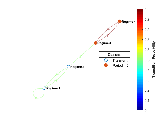
Mathematically, the probabilistic transition matrix characterizes the dynamics of the Markov chain. For more details, see Discrete-Time Markov Chains.
The variable st governs which state-specific submodel best describes yt during a particular period. Symbolically,
where:
is the dynamic regression model of yt in regime i.
xt is a vector of observed exogenous variables at time t.
θi is the collection of parameters of the submodel in regime i.
Markov-Switching Model Functionality of Econometrics Toolbox
The Econometrics Toolbox function msVAR
returns an msVAR object specifying the functional form and storing
the parameter values of a Markov-switching dynamic regression model for a univariate
or multivariate yt. An
msVAR object contains information about the structure of
st and the submodels for
yt. In addition to model
specification, the msVAR object framework enables you to fit models
to data and generate forecasts from models, among other common time series analysis
tasks.
Before you can create an msVAR object in MATLAB®, you must have the following information, which is application
dependent or based on economic theory:
The response variables yt to model.
A good statistical description of yt in each state. In other words, you need to know the structure of each submodel, which includes:
The presence of a model constant (intercept), but its value can be unknown
For multivariate models, the presence of a linear trend term
The autoregressive (AR) polynomial order
Predictor variables to include in the regression component
The number of states in the system.
A description of the state switching mechanism that determines how the submodels transition among each other. Although this topic uses a probabilistic discrete-time Markov chain for the switching mechanism, Econometrics Toolbox also supports fixed threshold transitions as the switching mechanism for a set of dynamic regression models. For more details, see Create Threshold-Switching Dynamic Regression Models.
The values of estimable parameters, such as model coefficients and the state transition matrix, can be known and specified or unknown and fit to data.
A time series plot of the response data can help you to understand the structure of the model. For example, consider building a simple dynamic model to forecast the US unemployment rate. The following figure shows a time series plot of the unemployment rate, with dark bands indicating periods of recession.
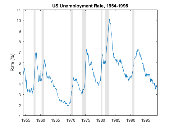
The plot shows relatively long periods during which the unemployment rate generally decreases and shorter periods during which the rate increases sharply. Those periods align with economic periods of expansion and recession, respectively. Within each state and across the sample, the dynamic behavior and volatility of the series appear similar. An autoregressive submodel for each economic state, expansion and recession, might capture the dynamics of the unemployment rate throughout the sample.
In summary, the plot suggests that a two-regime, switching system of autoregressive models for the unemployment rate series is plausible.
Represent Markov-Switching Model Using msVAR
To create a Markov-switching dynamic regression model, the msVAR
function requires these two inputs or property settings:
Submodels: A lengthNumStatesvector of state-specific linear autoregressive models describing the dynamics of yt. ThemsVARfunction accepts a vector completely composed of univariate autoregressive models (ARX,arimaobjects) or multivariate vector autoregression models (VARX,varmobjects), optionally containing an exogenous regression component. For more details, see Create Autoregressive (AR) Models, Create ARIMA Models That Include Exogenous Covariates, or Vector Autoregression (VAR) Model Creation.Switch: A discrete-time Markov chain that characterizes the probabilistic switching mechanism st among theNumStatesstates, specified as adtmcobject. The transition matrixSwitch.Pspecifies the switching probability distributions, in which elements are transition probabilities in the interval [0,1] or unknown (NaN) and fit to data. For more details on discrete-time Markov chains, see Markov Chain Modeling.
For example, create a Markov-switching dynamic regression model for the unemployment rate in the two-regime system. Assume AR(4) submodels for the rate in each state, and set all parameters to unknown values.
numStates = 2;
P = nan(numStates);
stateNames = ["Expansion" "Recession"];
mc = dtmc(P,StateNames=stateNames)
ar4 = arima(4,0,0);
mdl = [ar4; ar4];
Mdl1 = msVAR(mc,mdl)

transitionMatrix = Mdl1.Switch.P
submdl1 = Mdl1.Submodels(1)
mc =

  dtmc with properties:

             P: [2×2 double]
    StateNames: ["Expansion"    "Recession"]
     NumStates: 2

Mdl1 =

  msVAR with properties:

      NumStates: 2
      NumSeries: 1
     StateNames: ["Expansion"    "Recession"]
    SeriesNames: "1"
         Switch: [1×1 dtmc]
      Submodels: [2×1 varm]

transitionMatrix =

   NaN   NaN
   NaN   NaN

submdl1 =

  varm with properties:

     Description: "1-Dimensional VAR(4) Model"
     SeriesNames: "Y1"
       NumSeries: 1
               P: 4
        Constant: NaN
              AR: {NaNs} at lags [1 2 3 ... and 1 more]
           Trend: 0
            Beta: [1×0 matrix]
      Covariance: NaN
Although the elements of the input submodel vector are arima
objects, msVAR stores a vector of equivalent varm
objects. NaN-valued elements correspond to unknown, but
estimable, coefficient values or transition probabilities. You can treat all
estimable parameters as unknown or you can specify a mix of known and unknown
values. A model containing at least one unknown parameter is a partially
specified model. A partially specified model completely specifies the
model structure; its sole purpose is to specify which parameters the estimate
function should estimate. During estimation, specified parameter values indicate
equality constraints, but estimate always estimates innovations
covariances regardless of any specified values.
For example, suppose economic theory suggests that, during an expansion, AR lags 2 and 3 of the model are insignificant for the unemployment rate. Create a Markov-switching model to reflect this characteristic.
ar4adj = ar4;
ar4adj.AR(2:3) = {0}
Mdl2 = msVAR(mc,[ar4adj; ar4]);
ar4adj =

  arima with properties:

     Description: "ARIMA(4,0,0) Model (Gaussian Distribution)"
    Distribution: Name = "Gaussian"
               P: 4
               D: 0
               Q: 0
        Constant: NaN
              AR: {NaN NaN} at lags [1 4]
             SAR: {}
              MA: {}
             SMA: {}
     Seasonality: 0
            Beta: [1×0]
        Variance: NaN
Economic theory or a research hypothesis might suggest values for all parameters.
In this case, you can specify values of all model parameters, which results in a
fully specified model. You can pass a fully specified model
to any msVAR
object
function for further analysis. Also, to initiate the
expectation-maximization algorithm, estimate requires initial
values for all parameters. A fully specified model specifies the required initial
values.
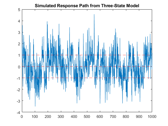
For example, create a simple three-regime model that uniformly switches between the following models, where εt is a standard Gaussian random variable:
yt = –1 + εt.
yt = εt.
yt = 1 + εt.
Simulate a 1000-period path from the model.
P = [0.9 0.1  0;
     0.25 0.5 0.25
     0    0.1 0.9];
mc3 = dtmc(P);
mdl1 = arima(Constant=-1,Variance=1);
mdl2 = arima(Constant=0,Variance=1);
mdl3 = arima(Constant=1,Variance=1);
mdlvec = [mdl1; mdl2; mdl3];
Mdl3 = msVAR(mc3,mdlvec);

rng("default") % For reproducibility
y = simulate(Mdl3,1000);

plot(y)
hold on
yline([-1 0 1],'r--')
title("Simulated Response Path from Three-State Model")
hold off