Transform Time Series Using Econometric Modeler App

The Econometric Modeler app enables you to transform time series data based on deterministic or stochastic trends you see in plots or hypothesis test conclusions. Available transformations in the app are log, seasonal and nonseasonal difference, and linear detrend. These examples show how to apply each transformation to time series data.

Apply Log Transformation to Data

This example shows how to stabilize a time series, whose variability grows with the level of the series, by applying the log transformation. The data set Data_Airline.mat contains monthly counts of airline passengers.

Download the Data_Airline.mat MAT-file into your current folder, and then load it into the workspace.

fldr = pwd;
openExample("Data_Airline.mat",workDir=fldr);
load(fullfile(fldr,"Data_Airline.mat"))

To change the folder to which to download the data set, set fldr to its absolute path.

At the command line, open the Econometric Modeler app.

econometricModeler

Alternatively, open the app from the apps gallery (see Econometric Modeler).

Import DataTimeTable into the app:

1. On the Modeler tab, in the Import section, click the Import button .

2. In the Import Data dialog box, select the check box for the DataTimeTable variable.

3. Click Import.

The variable PSSG appears in the Time Series pane, and its time series plot is in the Plot(PSSG) figure window.

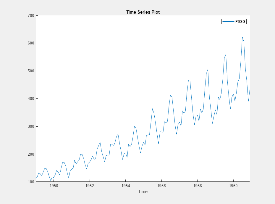
The series exhibits a seasonal trend, serial correlation, and possible exponential growth. For an interactive analysis of serial correlation, see Detect Serial Correlation Using Econometric Modeler App.

Apply the log transform to PSSG:

1. In the Time Series pane, select PSSG.

2. On the Modeler tab, in the Transforms section, click Log.

The transformed variable PSSG_Log appears in the Time Series pane, and its time series plot appears in the Plot(PSSG_Log) figure window.

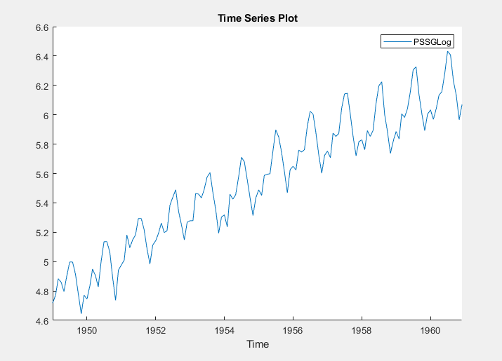
The exponential growth appears removed from the series.

Stabilize Time Series Using Nonseasonal Differencing

This example shows how to stabilize a time series by applying multiple nonseasonal difference operations. The data set, which is stored in Data_USEconModel.mat, contains the US gross domestic product (GDP) measured quarterly, among other series.

At the command line, load the Data_USEconModel.mat data set.

load Data_USEconModel

At the command line, open the Econometric Modeler app.

econometricModeler

Alternatively, open the app from the apps gallery (see Econometric Modeler).

Import DataTimeTable into the app:

1. On the Modeler tab, in the Import section, click the Import button .

2. In the Import Data dialog box, select the check box for the DataTimeTable variable.

3. Click Import.

The variables, including GDP, appear in the Time Series pane, and a time series plot of all the series appears in the Plot(COE) figure window.

In the Time Series pane, double-click GDP. A time series plot of GDP appears in the Plot(GDP) figure window.

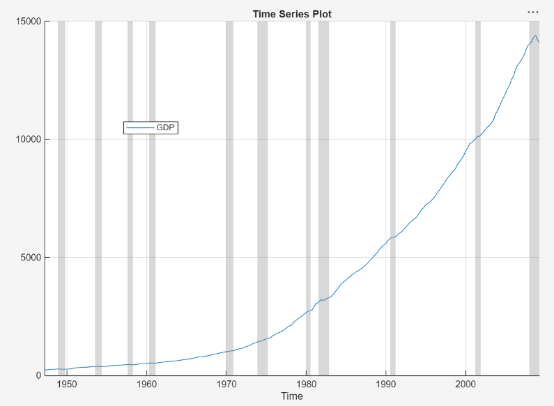
The series appears to grow without bound.

Apply the first difference to GDP. On the Modeler tab, in the Transforms section, click Difference.

In the Time Series pane, a variable representing the differenced GDP (GDP_Diff) appears. A time series plot of the differenced GDP appears in the Plot(GDP_Diff) figure window.

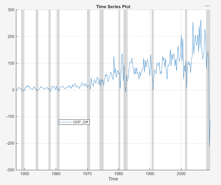
The differenced GDP series appears to grow without bound after 1970.

Apply the second difference to the GDP by differencing the differenced GDP. With GDP_Diff selected in the Time Series pane, on the Modeler tab, in the Transforms section, click Difference.

In the Time Series pane, a variable representing the transformed differenced GDP (GDP_Diff_Diff) appears. A time series plot of the differenced GDP appears in the Plot(GDP_Diff_Diff) figure window.

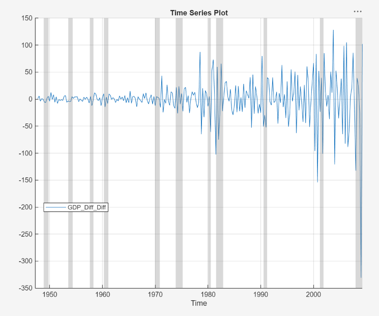
The transformed differenced GDP series appears stationary, although heteroscedastic.

Convert Prices to Returns

This example shows how to convert multiple series of prices to returns. The data set, which is stored in Data_USEconModel.mat, contains the US GDP and personal consumption expenditures measured quarterly, among other series.

At the command line, load the Data_USEconModel.mat data set.

load Data_USEconModel

At the command line, open the Econometric Modeler app.

econometricModeler

Alternatively, open the app from the apps gallery (see Econometric Modeler).

Import DataTimeTable into the app:

1. On the Modeler tab, in the Import section, click the Import button .

2. In the Import Data dialog box, select the check box for the DataTimeTable variable.

3. Click Import.

GDP and PCEC, among other series, appear in the Time Series pane, and a time series plot containing all series appears in the figure window.

In the Time Series pane, click GDP, then press Ctrl and click PCEC. Both series are selected.

Click the Plots tab, then click Time Series. A time series plot of GDP and PCEC appears in the Plot(GDP) figure window.

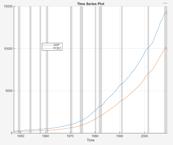
Both series, as prices, appear to grow without bound.

Convert the GDP and personal consumption expenditure prices to returns:

1. Click the Modeler tab. Ensure that GDP and PCEC are selected in the Time Series pane.

2. In the Transforms section, click Log.

   The Time Series pane displays variables representing the logged GDP series (GDPLog) and the logged personal consumption expenditure series (PCECLog).

3. With GDPLog and PCECLog selected in the Time Series pane, in the Transforms section, click Difference.

The Time Series pane displays variables representing the GDP returns (GDP_Log_Diff) and personal consumption expenditure returns (PCEC_Log_Diff). A time series plot of the GDP and personal consumption expenditure returns appears in the Plot(GDP_Log_Diff) figure window.

In the Time Series pane, rename the GDP_Log_Diff and PCEC_Log_Diff variables. Click GDP_Log_Diff twice to select its name and enter GDPReturns. Click PCEC_Log_Diff twice to select its name and enter PCECReturns.

The app updates the names of all documents associated with both returns.

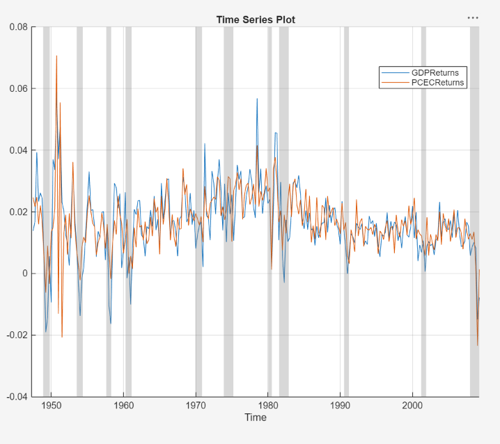
The series of GDP and personal consumption expenditure returns appear stationary, but observations within each series appear serially correlated.

Remove Seasonal Trend from Time Series Using Seasonal Difference

This example shows how to stabilize a time series exhibiting seasonal integration by applying a seasonal difference. The data set Data_Airline.mat contains monthly counts of airline passengers.

Download the Data_Airline.mat MAT-file into your current folder, and then load it into the workspace.

fldr = pwd;
openExample("Data_Airline.mat",workDir=fldr);
load(fullfile(fldr,"Data_Airline.mat"))

To change the folder to which to download the data set, set fldr to its absolute path.

At the command line, open the Econometric Modeler app.

econometricModeler

Alternatively, open the app from the apps gallery (see Econometric Modeler).

Import DataTimeTable into the app:

1. On the Modeler tab, in the Import section, click the Import button .

2. In the Import Data dialog box, select the check box for the DataTimeTable variable.

3. Click Import.

The variable PSSG appears in the Time Series pane, and its time series plot appears in the Plot(PSSG) figure window.

Address the seasonal trend by applying the 12th order seasonal difference. On the Modeler tab, in the Transforms section, set Seasonal to 12. Then, click Seasonal.

The transformed variable PSSG_SDiff appears in the Time Series pane, and its time series plot appears in the Plot(PSSG_SDiff) figure window.

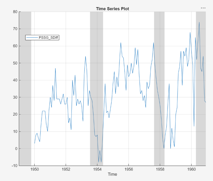
The transformed series appears to have a nonseasonal trend.

Address the nonseasonal trend by applying the first difference. With PSSG_SDiff selected in the Time Series pane, on the Modeler tab, in the Transforms section, click Difference.

The transformed variable PSSG_SDiff_Diff appears in the Time Series pane, and its time series plot appears in the Plot(PSSG_SDiff_Diff) figure window.

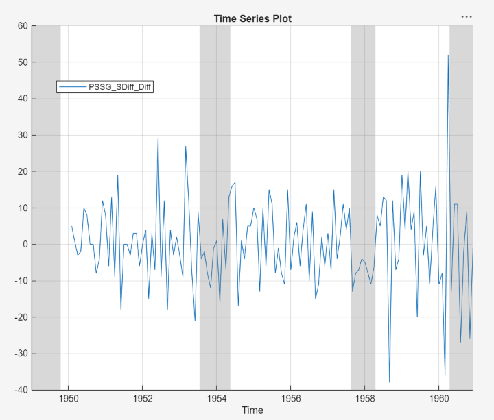
The transformed series appears stationary, but observations appear serially correlated.

In the Time Series pane, rename the PSSG_SDiff_Diff variable by clicking it twice to select its name and entering PSSGStable.

The app updates the names of all documents associated with the transformed series.

Remove Deterministic Trend from Time Series

This example shows how to remove a least-squares-derived deterministic trend from a nonstationary time series. The data set Data_Airline.mat contains monthly counts of airline passengers.

Download the Data_Airline.mat MAT-file into your current folder, and then load it into the workspace.

fldr = pwd;
openExample("Data_Airline.mat",workDir=fldr);
load(fullfile(fldr,"Data_Airline.mat"))

To change the folder to which to download the data set, set fldr to its absolute path.

At the command line, open the Econometric Modeler app.

econometricModeler

Alternatively, open the app from the apps gallery (see Econometric Modeler).

Import DataTimeTable into the app:

1. On the Modeler tab, in the Import section, click the Import button .

2. In the Import Data dialog box, select the check box for the DataTimeTable variable.

3. Click Import.

The variable PSSG appears in the Time Series pane, and its time series plot appears in the Plot(PSSG) figure window.

Apply the log transformation to the series. On the Modeler tab, in the Transforms section, click Log.

The transformed variable PSSG_Log appears in the Time Series pane, and its time series plot appears in the Plot(PSSG_Log) figure window.

Identify the deterministic trend by using least squares. Then, detrend the series by removing the identified deterministic trend. On the Modeler tab, in the Transforms section, click Detrend.

The transformed variable PSSG_Log_Detrend appears in the Time Series pane, and its time series plot appears in the Plot(PSSG_Log_Detrend) figure window.

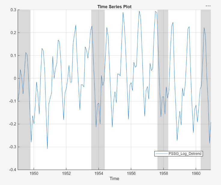
PSSG_Log_Detrend does not appear to have a deterministic trend, although it has a marked cyclic trend.