Compute Market Risk Capital Charge Using FRTB-SA Framework with CRR2
This example creates an frtbsa object and uses the ISDA® FRTB-SA framework to support workflows for calculating the capital market risk capital charge in accordance with the Capital Requirements Regulation 2 (CRR2). FRTB-SA (Standardized Approach for Fundamental Review of Trading Book) is a Basel Committee on Banking Supervision framework for calculating market capital risk requirements is based on CRR2, which extends the Basel regulations to include additional requirements for market risk, counterparty credit risk, and capital buffers specific to the EU.
To calculate the total market risk charge using CRR2, you need to use only the charge object function. However, for the purpose of illustration, this example also demonstrates the frtbsa object functions (sbm, drc, rrao).
Create frtbsa Object
format bankDefine the FRTB-SA CRIF file.
myCRIF = "FRTBSA_CRIF_CRR2.csv";Define the DRC reference date.
DrcRefCOBDate = datetime("21-Sep-2023");Create the FRTB-SA object in accordance with CRR2.
myFRTBSA = frtbsa(myCRIF, DRCValuationDate=DrcRefCOBDate, Regulation='CRR2')myFRTBSA =
frtbsa with properties:
CRIF: [159×18 table]
NumPortfolios: 2.00
PortfolioIDs: [2×1 string]
Portfolios: [2×1 frtbsa.Portfolio]
Regulation: "CRR2"
DomesticCurrency: "USD"
DRCValuationDate: 21-Sep-2023
NumDaysYear: 365.00
Examine Output
Display the contents of the FRTB-SA CRIF file.
myFRTBSA.CRIF
ans=159×18 table
    PortfolioID    TradeID       Variant       SensitivityID      RiskType      Qualifier     Bucket     Label1        Label2        Amount      AmountCurrency    AmountUSD    Label3    EndDate    CreditQuality    LongShortInd    CoveredBondInd    TrancheThickness
    ___________    ________    ____________    _____________    ____________    __________    ______    _________    ___________    _________    ______________    _________    ______    _______    _____________    ____________    ______________    ________________

       "P1"        "EQD_a1"    <missing>        "P1_EQD_a1"     "EQ_DELTA"      "ISSUER A"     "1"      <missing>    "SPOT"           8250.00        "USD"           8250.00     NaN        NaT        <missing>       <missing>        <missing>             NaN
       "P1"        "EQD_a2"    <missing>        "P1_EQD_a2"     "EQ_DELTA"      "ISSUER A"     "1"      <missing>    "REPO"           8333.33        "USD"           8333.33     NaN        NaT        <missing>       <missing>        <missing>             NaN
       "P1"        "EQD_b1"    <missing>        "P1_EQD_b1"     "EQ_DELTA"      "ISSUER B"     "2"      <missing>    "SPOT"          22000.00        "USD"          22000.00     NaN        NaT        <missing>       <missing>        <missing>             NaN
       "P1"        "EQV_a1"    "Variant 1"      "P1_EQV_a1"     "EQ_VEGA"       "ISSUER A"     "1"      "0.5"        <missing>         -50.00        "USD"            -50.00     NaN        NaT        <missing>       <missing>        <missing>             NaN
       "P1"        "EQV_a2"    "Variant 1"      "P1_EQV_a2"     "EQ_VEGA"       "ISSUER A"     "1"      "1"          <missing>         200.00        "USD"            200.00     NaN        NaT        <missing>       <missing>        <missing>             NaN
       "P1"        "EQV_b1"    "Variant 1"      "P1_EQV_b1"     "EQ_VEGA"       "ISSUER B"     "2"      "0.5"        <missing>        -166.67        "USD"           -166.67     NaN        NaT        <missing>       <missing>        <missing>             NaN
       "P1"        "EQC_a1"    "Variant 1a"     "P1_EQC_a1"     "EQ_CURV"       "ISSUER A"     "1"      "0.5"        <missing>      -18910.00        "USD"         -18910.00     NaN        NaT        <missing>       <missing>        <missing>             NaN
       "P1"        "EQC_a1"    "Variant 1a"     "P1_EQC_a1"     "EQ_CURV"       "ISSUER A"     "1"      "-0.5"       <missing>        6526.25        "USD"           6526.25     NaN        NaT        <missing>       <missing>        <missing>             NaN
       "P1"        "EQC_b1"    "Variant 1a"     "P1_EQC_b1"     "EQ_CURV"       "ISSUER B"     "2"      "0.5"        <missing>       -6288.00        "USD"          -6288.00     NaN        NaT        <missing>       <missing>        <missing>             NaN
       "P1"        "EQC_b1"    "Variant 1a"     "P1_EQC_b1"     "EQ_CURV"       "ISSUER B"     "2"      "-0.5"       <missing>        6120.00        "USD"           6120.00     NaN        NaT        <missing>       <missing>        <missing>             NaN
       "P1"        "CMD_a1"    <missing>        "P1_CMD_a1"     "COMM_DELTA"    "COAL"         "1"      "0"          "NEWCASTLE"      2000.00        "USD"           2000.00     NaN        NaT        <missing>       <missing>        <missing>             NaN
       "P1"        "CMD_a2"    <missing>        "P1_CMD_a2"     "COMM_DELTA"    "COAL"         "1"      "0"          "LONDON"         -500.00        "USD"           -500.00     NaN        NaT        <missing>       <missing>        <missing>             NaN
       "P1"        "CMD_b1"    <missing>        "P1_CMD_b1"     "COMM_DELTA"    "BRENT"        "2"      "0"          "LE HAVRE"        666.67        "USD"            666.67     NaN        NaT        <missing>       <missing>        <missing>             NaN
       "P1"        "CMD_c1"    <missing>        "P1_CMD_c1"     "COMM_DELTA"    "WTI"          "2"      "2"          "OKLAHOMA"       -875.00        "USD"           -875.00     NaN        NaT        <missing>       <missing>        <missing>             NaN
       "P1"        "CMV_a1"    "Variant 1"      "P1_CMV_a1"     "COMM_VEGA"     "COAL"         "1"      "0.5"        <missing>         333.33        "USD"            333.33     NaN        NaT        <missing>       <missing>        <missing>             NaN
       "P1"        "CMV_a2"    "Variant 1"      "P1_CMV_a2"     "COMM_VEGA"     "COAL"         "1"      "1"          <missing>        -100.00        "USD"           -100.00     NaN        NaT        <missing>       <missing>        <missing>             NaN
      ⋮
Display the number of portfolios and their IDs.
myFRTBSA.NumPortfolios
ans =
          2.00
myFRTBSA.PortfolioIDs
ans = 2×1 string
    "P1"
    "P2"
Display the properties of the first Portfolio object.
myFRTBSA.Portfolios(1)
ans =
  Portfolio with properties:

    PortfolioID: "P1"
         Trades: [69×1 frtbsa.Trade]
      RiskTypes: [69×1 string]
Display RiskTypes of the portfolio.
myFRTBSA.Portfolios(1).RiskTypes
ans = 69×1 string
    "EQ_DELTA"
    "EQ_DELTA"
    "EQ_DELTA"
    "EQ_VEGA"
    "EQ_VEGA"
    "EQ_VEGA"
    "EQ_CURV"
    "EQ_CURV"
    "COMM_DELTA"
    "COMM_DELTA"
    "COMM_DELTA"
    "COMM_DELTA"
    "COMM_VEGA"
    "COMM_VEGA"
    "COMM_VEGA"
    "COMM_VEGA"
    "COMM_CURV"
    "COMM_CURV"
    "COMM_CURV"
    "GIRR_DELTA"
    "GIRR_DELTA"
    "GIRR_DELTA"
    "GIRR_VEGA"
    "GIRR_VEGA"
    "GIRR_VEGA"
    "GIRR_CURV"
    "GIRR_CURV"
    "FX_DELTA"
    "FX_DELTA"
    "FX_VEGA"
      ⋮
Display some of the trades of the portfolio.
myFRTBSA.Portfolios(1).Trades(1)
ans =
  Trade with properties:

             TradeID: "EQD_a1"
             Variant: <missing>
       SensitivityID: "P1_EQD_a1"
            RiskType: "EQ_DELTA"
           Qualifier: "ISSUER A"
              Bucket: "1"
              Label1: <missing>
              Label2: "SPOT"
              Amount: 8250.00
      AmountCurrency: "USD"
           AmountUSD: 8250.00
              Label3: NaN
             EndDate: NaT
       CreditQuality: <missing>
        LongShortInd: <missing>
      CoveredBondInd: <missing>
    TrancheThickness: NaN
myFRTBSA.Portfolios(1).Trades(30)
ans =
  Trade with properties:

             TradeID: "FXV_b1"
             Variant: "Variant 1"
       SensitivityID: "P1_FXV_b1"
            RiskType: "FX_VEGA"
           Qualifier: "EURCLP"
              Bucket: <missing>
              Label1: "0.5"
              Label2: <missing>
              Amount: 175.00
      AmountCurrency: "USD"
           AmountUSD: 175.00
              Label3: NaN
             EndDate: NaT
       CreditQuality: <missing>
        LongShortInd: <missing>
      CoveredBondInd: <missing>
    TrancheThickness: NaN
myFRTBSA.Portfolios(1).Trades(60)
ans =
  Trade with properties:

             TradeID: "RRAO_a2"
             Variant: <missing>
       SensitivityID: "P1_RRAO_a2"
            RiskType: "RRAO_01_PERCENT"
           Qualifier: <missing>
              Bucket: <missing>
              Label1: <missing>
              Label2: <missing>
              Amount: 300000.00
      AmountCurrency: "USD"
           AmountUSD: 300000.00
              Label3: NaN
             EndDate: NaT
       CreditQuality: <missing>
        LongShortInd: <missing>
      CoveredBondInd: <missing>
    TrancheThickness: NaN
Compute Market Risk Capital Charge
The charge is the sum of the capital charges for all risk factor categories, plus any applicable add-ons. Use charge to compute the capital market risk charge for all portfolios in the frtbsa object.
ChargeResults = charge(myFRTBSA)
ChargeResults =
  chargeResults with properties:

       NumPortfolios: 2.00
        PortfolioIDs: [2×1 string]
          Regulation: "CRR2"
    DomesticCurrency: "USD"
             Charges: [2×1 double]
    ComponentResults: [2×1 frtbsa.chargePortfolioResults]
        ResultsTable: [2×5 table]
The Charges output contains the capital risk charge of the portfolios.
ChargeResults.Charges
ans = 2×1

     299048.97
     170592.48
The ResultsTable output contains the high-level risk charge calculations of the portfolios: total portfolio charge, RRAO charge, DRC charge, and SBM charge.
ChargeResults.ResultsTable
ans=2×5 table
    PortfolioID      Total       RRAO         DRC          SBM
    ___________    _________    _______    _________    _________

       "P1"        299048.97    3310.00    171008.51    124730.46
       "P2"        170592.48    2800.00     45024.29    122768.19
The ComponentResults output contains detailed capital risk charge information for a given portfolio. Examine the market risk capital charge for the second portfolio.
ChargeResults.ComponentResults(2)
ans =
  chargePortfolioResults with properties:

    PortfolioID: "P2"
         Charge: 170592.48
            SBM: [1×1 frtbsa.sbmPortfolioResults]
            DRC: [1×1 frtbsa.drcPortfolioResults]
           RRAO: [1×1 frtbsa.rraoPortfolioResults]
Examine the SBM component of this portfolio.
ChargeResults.ComponentResults(2).SBM
ans =
  sbmPortfolioResults with properties:

            PortfolioID: "P2"
                 Charge: 122768.19
    ChargeByCorrelation: [1×1 struct]
      ChargeByRiskClass: [21×5 table]
     IntrabucketCharges: [1×1 struct]
Display charges by risk class.
ChargeResults.ComponentResults(2).SBM.ChargeByRiskClass
ans=21×5 table
    RiskClass    RiskMeasure    LowCorrelation    MediumCorrelation    HighCorrelation
    _________    ___________    ______________    _________________    _______________

    "GIRR"       "Delta"             296.23             298.38              300.52
    "GIRR"       "Vega"              316.67             316.67              316.67
    "GIRR"       "Curvature"        9323.83            9323.83             9323.83
    "CSR_NS"     "Delta"              62.47              62.48               62.50
    "CSR_NS"     "Vega"               47.79              47.24               46.67
    "CSR_NS"     "Curvature"         393.90             393.90              393.90
    "CSR_SC"     "Delta"             524.62             552.15              578.37
    "CSR_SC"     "Vega"              226.09             236.62              246.70
    "CSR_SC"     "Curvature"       39765.25           39809.40            39853.51
    "CSR_SNC"    "Delta"             455.99             456.10              456.21
    "CSR_SNC"    "Vega"              489.20             498.11              506.86
    "CSR_SNC"    "Curvature"       19206.41           19206.41            19206.41
    "FX"         "Delta"               8.84               8.84                8.84
    "FX"         "Vega"              150.00             150.00              150.00
    "FX"         "Curvature"       21373.78           21373.78            21373.78
    "EQ"         "Delta"           14432.78           14587.58            14740.74
      ⋮
Examine the DRC component of this portfolio.
ChargeResults.ComponentResults(2).DRC
ans =
  drcPortfolioResults with properties:

            PortfolioID: "P2"
                 Charge: 45024.29
    ChargeByCreditClass: [2×2 table]
     IntrabucketCharges: [1×1 struct]
Display charges by credit class.
ChargeResults.ComponentResults(2).DRC.ChargeByCreditClass
ans=2×2 table
    CreditClass     Charge
    ___________    ________

       "NS"        14750.00
       "SNC"       30274.29
Examine the RRAO component of this portfolio.
ChargeResults.ComponentResults(2).RRAO
ans =
  rraoPortfolioResults with properties:

               PortfolioID: "P2"
                    Charge: 2800.00
     ChargeBySensitivityID: [2×5 table]
    ChargeByInstrumentType: [2×2 table]
Display charges by instrument type.
ChargeResults.ComponentResults(2).RRAO.ChargeByInstrumentType
ans=2×2 table
    InstrumentType    Charge
    ______________    _______

       "Exotic"       2500.00
       "ORR"           300.00
Use the chargeChart function to plot the total capital market risk charge for each portfolio.
chargeChart(myFRTBSA,Style = "final")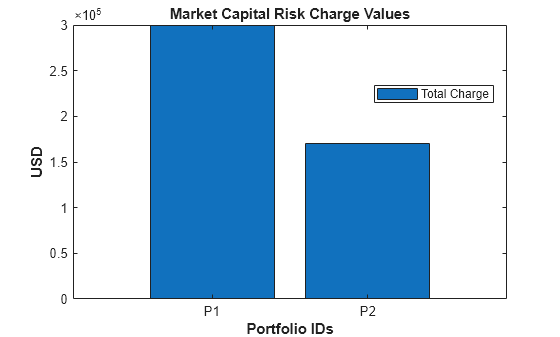
Compute DRC Charge
The default risk capital (DRC) charge captures the risk of default of issuers of debt and equity instruments in the trading book. Use drc with the frtbsa object to compute the DRC charge for each portfolio.
DRCResults = drc(myFRTBSA)
DRCResults =
  drcResults with properties:

       NumPortfolios: 2.00
        PortfolioIDs: [2×1 string]
          Regulation: "CRR2"
    DomesticCurrency: "USD"
             Charges: [2×1 double]
    ComponentResults: [2×1 frtbsa.drcPortfolioResults]
        ResultsTable: [2×4 table]
The Charges output contains the DRC risk charge of the portfolios.
DRCResults.Charges
ans = 2×1

     171008.51
      45024.29
The ResultsTable output contains the high-level risk DRC charge calculations of the portfolios.
DRCResults.ResultsTable
ans=2×4 table
    PortfolioIDs      Total         NS          SNC
    ____________    _________    ________    _________

        "P1"        171008.51    14750.00    156258.51
        "P2"         45024.29    14750.00     30274.29
The ComponentResults output contains detailed DRC risk charge information for a given portfolio. Examine the DRC risk charge for the first portfolio.
DRCResults.ComponentResults(1)
ans =
  drcPortfolioResults with properties:

            PortfolioID: "P1"
                 Charge: 171008.51
    ChargeByCreditClass: [2×2 table]
     IntrabucketCharges: [1×1 struct]
Display the charges by credit class. Portfolio P1 has non-securitization and securitization non-correlation trading portfolio (CTP) trades.
DRCResults.ComponentResults(1).ChargeByCreditClass
ans=2×2 table
    CreditClass     Charge
    ___________    _________

       "NS"         14750.00
       "SNC"       156258.51
Display the intrabucket charges for the non-securitization trades.
DRCResults.ComponentResults(1).IntrabucketCharges.NS
ans=2×4 table
       Bucket       NetLongJtd    NetShortJdt     Charge
    ____________    __________    ___________    ________

    "CORPORATES"     12750.00        0.00        12750.00
    "SOVEREIGNS"      2000.00        0.00         2000.00
Display the intrabucket charges for the securitization non-CTP trades.
DRCResults.ComponentResults(1).IntrabucketCharges.SNC
ans=1×9 table
       Bucket       NonSeniorLongJtd    NonSeniorShortJtd    SeniorLongJtd    SeniorShortJtd    NetLongJtd    NetShortJtd    HBR      Charge
    ____________    ________________    _________________    _____________    ______________    __________    ___________    ____    _________

    "CORPORATES"          0.00                0.00             746666.67        -300000.00      746666.67      300000.00     0.71    156258.51
Use the drcChart function to plot the DRC charges for each portfolio.
drcChart(myFRTBSA,Style="final")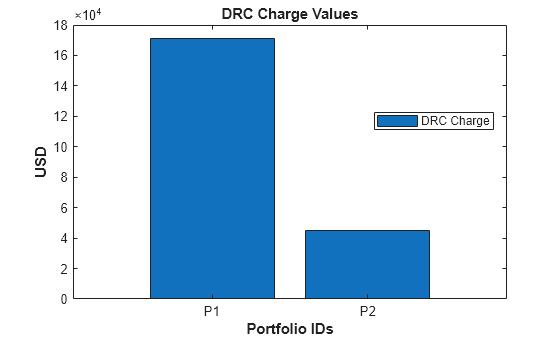
Compute RRAO Capital Charge
The residual risk add-on (RRAO) charge covers risks that are not fully captured by the other components of the FRTB capital charges, particularly those arising from positions with exotic or nonlinear payoffs, as well as other risks that are residual in nature. Use rrao with the frtbsa object to compute the RRAO charge results for each portfolio.
RRAOResults = rrao(myFRTBSA)
RRAOResults =
  rraoResults with properties:

       NumPortfolios: 2.00
        PortfolioIDs: [2×1 string]
          Regulation: "CRR2"
    DomesticCurrency: "USD"
             Charges: [2×1 double]
    ComponentResults: [2×1 frtbsa.rraoPortfolioResults]
        ResultsTable: [2×4 table]
The Charges output contains the RRAO risk charge of the portfolios.
RRAOResults.Charges
ans = 2×1

       3310.00
       2800.00
The ResultsTable output contains the high-level risk RRAO charge calculations of the portfolios.
RRAOResults.ResultsTable
ans=2×4 table
    PortfolioIDs     Total     Exotic      ORR
    ____________    _______    _______    ______

        "P1"        3310.00    3000.00    310.00
        "P2"        2800.00    2500.00    300.00
The ComponentResults output contains detailed RRAO risk charge information for a given portfolio. Examine the RRAO risk charge for the first portfolio.
RRAOResults.ComponentResults(1)
ans =
  rraoPortfolioResults with properties:

               PortfolioID: "P1"
                    Charge: 3310.00
     ChargeBySensitivityID: [4×5 table]
    ChargeByInstrumentType: [2×2 table]
Display charges by instrument type. Portfolio P1 has both exotic underlying instruments and other residual risk instruments.
RRAOResults.ComponentResults(1).ChargeByInstrumentType
ans=2×2 table
    InstrumentType    Charge
    ______________    _______

       "Exotic"       3000.00
       "ORR"           310.00
Use the rraoChart function to plot the RRAO capital charges for each portfolio.
rraoChart(myFRTBSA,Style="final")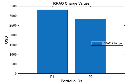
Compute SBM Capital Charge
Under the sensitivity-based market (SBM), banks calculate capital charges based on the sensitivities of their trading book positions to various risk factors. Use sbm with the frtbsa object to compute the SBM charge results for each portfolio.
SBMResults = sbm(myFRTBSA)
SBMResults =
  sbmResults with properties:

       NumPortfolios: 2.00
        PortfolioIDs: [2×1 string]
          Regulation: "CRR2"
    DomesticCurrency: "USD"
             Charges: [2×1 double]
    ComponentResults: [2×1 frtbsa.sbmPortfolioResults]
        ResultsTable: [2×10 table]
The Charges output contains the SBM risk charge of the portfolios.
SBMResults.Charges
ans = 2×1

     124730.46
     122768.19
The ResultsTable output contains the high-level risk SBM charge calculations of the portfolio.
SBMResults.ResultsTable
ans=2×10 table
    PortfolioID    Correlation      Total        GIRR      CSR_NS     CSR_SC     CSR_SNC        FX          EQ        COMM
    ___________    ___________    _________    ________    ______    ________    ________    ________    ________    _______

       "P1"          "high"       124730.46    10183.45    772.91    40678.57    20169.47    21532.62    23991.46    7401.98
       "P2"          "high"       122768.19     9941.02    503.07    40678.57    20169.47    21532.62    23954.45    5988.99
The ComponentResults output contains detailed SBM risk charge information for a given portfolio. Examine the SBM risk charge for the first portfolio.
SBMResults.ComponentResults(1)
ans =
  sbmPortfolioResults with properties:

            PortfolioID: "P1"
                 Charge: 124730.46
    ChargeByCorrelation: [1×1 struct]
      ChargeByRiskClass: [21×5 table]
     IntrabucketCharges: [1×1 struct]
Display charges by risk class.
SBMResults.ComponentResults(1).ChargeByRiskClass
ans=21×5 table
    RiskClass    RiskMeasure    LowCorrelation    MediumCorrelation    HighCorrelation
    _________    ___________    ______________    _________________    _______________

    "GIRR"       "Delta"             334.39             338.69              342.95
    "GIRR"       "Vega"              514.22             515.45              516.67
    "GIRR"       "Curvature"        9323.83            9323.83             9323.83
    "CSR_NS"     "Delta"              99.59             105.32              110.75
    "CSR_NS"     "Vega"              148.40             154.95              161.24
    "CSR_NS"     "Curvature"         469.33             485.38              500.92
    "CSR_SC"     "Delta"             524.62             552.15              578.37
    "CSR_SC"     "Vega"              226.09             236.62              246.70
    "CSR_SC"     "Curvature"       39765.25           39809.40            39853.51
    "CSR_SNC"    "Delta"             455.99             456.10              456.21
    "CSR_SNC"    "Vega"              489.20             498.11              506.86
    "CSR_SNC"    "Curvature"       19206.41           19206.41            19206.41
    "FX"         "Delta"               8.84               8.84                8.84
    "FX"         "Vega"              150.00             150.00              150.00
    "FX"         "Curvature"       21373.78           21373.78            21373.78
    "EQ"         "Delta"           14451.94           14608.10            14762.60
      ⋮
Display the low correlation scenario charges.
SBMResults.ComponentResults(1).ChargeByCorrelation.Low
ans=8×4 table
                Delta       Vega      Curvature     Charge
               ________    _______    _________    _________

    GIRR         334.39     514.22      9323.83     10172.44
    CSR_NS        99.59     148.40       469.33       717.31
    CSR_SC       524.62     226.09     39765.25     40515.96
    CSR_SNC      455.99     489.20     19206.41     20151.60
    FX             8.84     150.00     21373.78     21532.62
    EQ         14451.94     165.09      9021.88     23638.91
    COMM         464.34     238.26      6459.15      7161.74
    Total      16339.70    1931.26    105619.63    123890.59
Display the intrabucket charges for this portfolio for the equity class and the delta risk sensitivity.
SBMResults.ComponentResults(1).IntrabucketCharges.EQ.Delta
ans=2×5 table
    Bucket       Sb       LowCorrelation    MediumCorrelation    HighCorrelation
    ______    ________    ______________    _________________    _______________

     1.00      4583.33        4583.24            4583.29             4583.33
     2.00     13200.00       13200.00           13200.00            13200.00
Display the intrabucket charges for this portfolio for the GIRR class and the vega risk sensitivity.
SBMResults.ComponentResults(1).IntrabucketCharges.GIRR.Vega
ans=1×5 table
    Bucket      Sb      LowCorrelation    MediumCorrelation    HighCorrelation
    ______    ______    ______________    _________________    _______________

    "USD"     516.67        514.22             515.45              516.67
Use the sbmChart function to plot the SBM charge for each portfolio.
sbmChart(myFRTBSA,Style="final")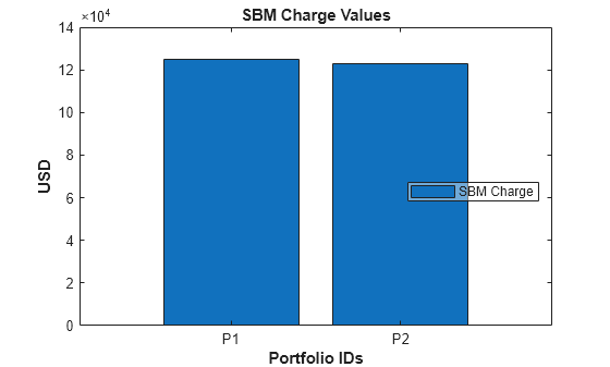
See Also
frtbsa | charge | sbm | drc | rrao | saccr