Model an Ice Maker by Using Mode Charts in a Custom Simscape Block

This example shows how to model an ice maker in Simscape™ by designing a custom block that uses mode charts to represent freezing water in the machine. You create a model that represents the refrigeration cycle and the ice compartment. Then, you create a custom Simscape block that uses a mode chart to model the states of the water, from liquid to solid. For more information about mode charts, see Mode Chart Modeling.

Design the Ice Maker

The ice maker freezes water in 0.9 L batches. Each batch starts at 298.15 K and freezes inside the compartment at 255 K. The ambient air outside the ice maker stays at 298.15 K.

Specify Ice Compartment Geometry and Thermal Characteristics

The ice maker consists of a refrigeration cycle and an ice compartment. The freezing water is in an ice tray within the ice compartment. Specify parameters that define the ice compartment, tray geometry, and their thermal properties:

h_tray = 0.03; % [m] Height of ice tray
w_tray = 0.3; % [m] Width of ice tray
d_tray = 0.1; % [m] Depth of ice tray
t_tray = 0.002; % [m] Thickness of ice tray wall
V_water = h_tray * w_tray * d_tray; % [m^3] Volume of freezing water

k_tray = 0.2; % [W/m*K] Thermal resistivity of ice tray wall
Cp_tray = 20; % [kJ/kg*K] Specific heat capacity of ice tray wall
rho_tray = 1000; % [kg/m^3] Density of ice tray wall

h_compartment = 0.5; % [m] Height of ice compartment
w_compartment = 0.3; % [m] Width of ice compartment
d_compartment = 0.4; % [m] Depth of ice compartment
t_compartment = 0.05; % [m] Thickness of ice compartment wall

k_compartment = 0.02; % [W/m*K] Thermal conductivity of ice compartment wall
Cp_compartment = 1500; % [kJ/kg*K] Specific heat capacity of ice compartment wall
rho_compartment = 30; % [kg/m^3] Density of ice compartment wall

h_stillAir = 5; % [W/m^2*K] Heat transfer coefficient of still air
h_blownAir = 30; % [W/m^2*K] Heat transfer coefficient of blown air

Calculate Refrigeration Requirements

Next, calculate the heat that the refrigeration cycle must remove to freeze the water. This value depends on the thermodynamic properties and mass of each batch of water. First, define the relevant thermophysical properties of the water:

rho_liquid = 997; % [kg/m^3} Density of water
Cp_liquid = 4.184; % [kJ/kg*K] Specific heat capacity of liquid water
dH_fusion = 334; % [kJ/kg] Latent heat of fusion of water
T_initial = 298.15; % [K] Initial temperature of water
T_freezing = 273.15; % [K] Freezing temperature of water at 1 atm
T_environment = 298.15; % [K] Temperature of ambient environment outside ice maker
T_set = 255; % [K] Ice compartment temperature set point

Calculate the mass of water in each batch and the temperature difference between the initial and freezing temperatures of the water.

m_water = V_water * rho_liquid; % [kg] Mass of water
dT_cooling = T_freezing - T_initial; % [K] Temperature change to freezing

Next, compute the total heat the ice maker must remove to freeze each batch of water. This value includes the sensible heat and the latent heat of fusion,

$$Q_{freeze}=\Delta H_{freeze}=m_{water}\left(C_{p,l}\Delta T_{cooling}-\Delta H_f\right)$$,

where:

• $$Q_{freeze}$$ is the heat required to freeze the water.

• $$\Delta H_{freeze}$$ is the change in enthalpy of cooling and freezing the water.

• $$m_{water}$$ is the mass of each batch of water.

• $$C_{P,l}$$ is the specific heat capacity of liquid water.

• $$\Delta T_{cooling}$$ is the difference between the initial temperature of the water and its freezing temperature.

• $$\Delta H_f$$ is the latent heat of fusion of water.

dH_freeze = m_water * (Cp_liquid * dT_cooling - dH_fusion); % [kJ] Enthalpy change to freeze one batch
Q_freeze = dH_freeze; % [kJ] Heat of freezing

Calculate the cooling rate,

$${\underset{}{\overset{\dot{}}{Q}}}_{freeze}=\frac{Q_{freeze}}{\Delta t}$$,

where a dot represents a rate per time.

dt_freeze = 7200; % [s] Estimated time to freeze one batch of ice
Qdot_freeze = Q_freeze / dt_freeze % [kW] Cooling rate for freezing

Qdot_freeze = 
-0.0547

Design the refrigeration cycle

Next, use the cooling requirement to design the refrigeration cycle. Start by defining the subcooling and superheat margins.

dT_subcooling = 10; % [K] Subcooling
dT_superheating = 10; % [K] Superheating

To understand how the refrigerant behaves, use a pressure-enthalpy (P-H) diagram for R-134a. To view a P-H diagram, you can open an empty model, add a Two-Phase Fluid Predefined Properties (2P) block, and double-click on the block to open the block dialog. Set Two-phase fluid to R-134a. In the Plots section, click the Plot button for the Two-phase fluid properties (contours). In the plot window, in the top-left corner, click the Enthalpy-x-axis button.

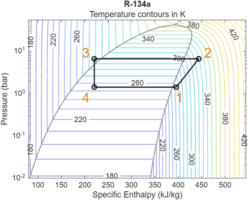
Using the design specifications, select four key points on the diagram:

1. Evaporator outlet

2. Compressor outlet

3. Condenser outlet

4. Expansion valve outlet

These points define the thermodynamic cycle. For more information about how you select these four points, see Model a Refrigeration Cycle. Use the enthalpy values at these points to calculate the coefficient of performance (COP),

$$COP=\frac{h_1-h_4}{h_2-h_1}$$,

where $$h_1$$, $$h_2$$, $$h_3$$, and $$h_4$$ are the enthalpies of the refrigerant at points 1 through 4.

h1 = 395.7; % [kJ/kg] Enthalpy at point 1
h2 = 443.7; % [kJ/kg] Enthalpy at point 2
h3 = 227.5; % [kJ/kg] Enthalpy at point 3
h4 = 227.5; % [kJ/kg] Enthalpy at point 4
COP = (h1 - h4) / (h2 - h1) % Coefficient of Performance

COP = 
3.5042

The evaporator removes heat at a rate equal to the cooling rate of freezing water when the ice maker is perfectly insulated:

$${\underset{}{\overset{\dot{}}{Q}}}_{evap}={\underset{}{\overset{\dot{}}{Q}}}_{freeze}$$,

$$\underset{}{\overset{\dot{}}{W}}=\frac{{\underset{}{\overset{\dot{}}{Q}}}_{evap}}{COP}$$,

$${\underset{}{\overset{\dot{}}{Q}}}_{cond}={\underset{}{\overset{\dot{}}{Q}}}_{evap}+\underset{}{\overset{\dot{}}{W}}$$,

where:

• $${\underset{}{\overset{\dot{}}{Q}}}_{evap}$$ is the heat load of the evaporator.

• $$\underset{}{\overset{\dot{}}{W}}$$ is the work rate of the refrigeration cycle.

• $${\underset{}{\overset{\dot{}}{Q}}}_{cond}$$ is the heat load of the condenser.

Qdot_evap = Qdot_freeze; % [kJ/hr] Heat rate of evaporator
Wdot = Qdot_evap / COP % [kJ/hr] External work requirement to refrigeration cycle

Wdot = 
-0.0156

Qdot_cond = Qdot_evap + Wdot % [kJ/hr] Heat rate of condenser

Qdot_cond = 
-0.0703

You can use these heat rates to calculate the mass flow rates of air through the condenser and evaporator,

$$\underset{}{\overset{\dot{}}{m}}=\frac{\underset{}{\overset{\dot{}}{Q}}}{C_{p,air}\Delta T}$$,

where:

• $$\underset{}{\overset{\dot{}}{m}}$$ is the mass flow rate of air for the condenser or evaporator.

• $$\underset{}{\overset{\dot{}}{Q}}$$ is the heat load for the condenser or evaporator.

• $$C_{p,air}$$ is the specific heat capacity of air.

Cp_air = 1.00; % [kJ/kg*K] Specific heat capacity of air
dT_evap = 10; % [K] Temperature drop of air across evaporator
dT_cond = 10; % [K] Temperature drop of air across compressor
mdot_evap = Qdot_evap / (Cp_air * dT_evap) % [kg/hr] Mass flow rate of air through evaporator

mdot_evap = 
-0.0055

mdot_cond = Qdot_cond / (Cp_air * dT_cond) % [kg/hr] Mass flow rate of air through compressor

mdot_cond = 
-0.0070

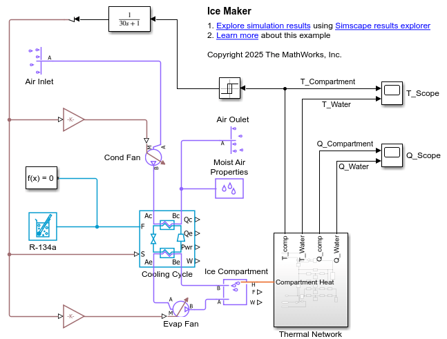
Build the Model

Next, build a model to represent the ice maker. The model includes three domains:

• A two-phase fluid domain for the refrigerant,

• A thermal domain for heat flow,

• A moist air domain for the air inside the compartment and the surrounding environment.

It also includes a custom block that models freezing water and the effect of the water on the rest of the ice maker.

Model the Refrigeration Cycle

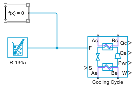
1. Open the model you created with a Two-Phase Fluid Predefined Properties (2P) block. Add a System-Level Refrigeration Cycle (2P) block to model the refrigeration cycle.

2. Open the System-Level Refrigeration Cycle (2P) block and set Pressure specification to Pressure at specified saturation temperature.

3. Set the block parameters to match the specifications above. Set Nominal condensing (saturation) temperature to T_environment + dT_subcooling + 5 and Nominal evaporating (saturation) temperature to T_set - dT_superheat - 5.

4. Connect the Two-Phase Fluid Predefined Properties (2P) block to port F of the System-Level Refrigeration Cycle (2P) block.

5. Add and connect a Solver Configuration block.

To ensure the condenser expels heat into the ambient environment, verify that the value of the Condenser External Fluid Nominal inlet temperature is less than the condenser refrigerant outlet temperature. The condenser refrigerant outlet temperature is equal to the value of the Nominal condensing (saturation) temperature minus the Nominal condenser subcooling. To ensure the evaporator can absorb heat, verify that the value of the Evaporator External Fluid Nominal inlet temperature is greater than the evaporator refrigerant outlet temperature. The evaporator refrigerant outlet temperature is equal to the value of the Nominal evaporating (saturation) temperature plus the Nominal (static + opening) evaporator superheat.

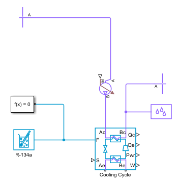
Model the Ambient Environment

1. Add a Reservoir (MA) block. This block represents the environment.

2. In the block set Reservoir temperature specification to Specified temperature and set Reservoir temperature to T_environment K.

3. Add a Flow Rate Source (MA) block and connect port A to the Reservoir (MA) block. Connect port B to port Ac of the System-Level Refrigeration Cycle (2P) block.

4. Copy the Reservoir (MA) block and connect it to port Bc of the System-Level Refrigeration Cycle (2P) block.

5. Add and connect a Moist Air Properties block to the moist air network.

Build the Ice Compartment

Use the moist air and thermal domains to model the ice compartment. Create a custom Simscape block to model the freezing water and its effects on the ice maker.

1. Add a Flow Rate Source (MA) block and connect port A to port Ae of the System-Level Refrigeration Cycle (2P) block.

2. Add a Constant Volume Chamber (MA) block. This block represents the air in the ice compartment. Open the block and set Number of ports to 2.

3. Set Chamber volume to w_compartment * d_compartment * h_compartment m^3.

4. Connect port A of the Constant Volume Chamber (MA) block to port B of the Flow Rate Source (MA) block.

5. Connect port B to port Be of the System-Level Refrigeration Cycle (2P) block.

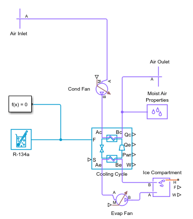
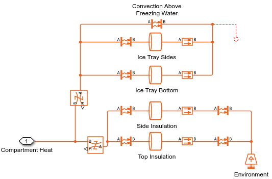
Next, build the ice maker thermal network and connect it to port H of the Constant Volume Chamber (MA) block. The thermal network models heat transfer from the ambient environment to the ice compartment. Include an unconnected physical signal in the model to connect to the custom Simscape block. In this system, the:

• Thermal Mass blocks model the solids in the thermal network like the ice compartment walls and the ice tray walls

• Convective Heat Transfer blocks model the convective heat transfer from the air to the solids in the thermal network

• Conductive Heat Transfer blocks model the heat conduction through the solids in the thermal network

Create a Custom Simscape Block

You can use the Simscape language to create a custom block that models the discontinuous thermodynamic properties of freezing water. For more information about creating custom Simscape blocks, see Creating Custom Components. For this example, open the freezingWater.ssc file:

open('freezingWater.ssc')

This file uses the modecharts construct to represent freezing and melting water:

• The modecharts construct defines the thermal properties and handles the phase changes in the water.

• The liquidPhase section contains the equations that describe the water when it is in the liquid state. The liquid fraction, x, is 1 during this phase. The temperature of the block changes in proportion to the rate of heat flow to or from the block.

• The phaseChange section contains the equations that describe the water when it is freezing or melting. The temperature of the block does not change during this phase. All heat flow into or out of the block contributes to changes in the liquid fraction, x.

• The solidPhase section contains the equations that describe the water when it is in the solid state. The liquid fraction, x, is 0 during this phase. The temperature of the block changes in proportion to the rate of heat flow to or from the block.

Complete the thermal network by adding the custom Simscape block using the Simscape Component block, Temperature Sensor blocks to measure the temperature of the ice compartment and freezing water, and Outport and PS-Simulink Converter blocks to pass Simulink signals out of the subsystem. Name the subsystem Thermal Network.

Add Control Feedback and Scopes

1. To view the temperature and heat flow in the ice compartment, add two Scope blocks and name them T_scope and Q_Scope.

2. Add a Relay block and connect the input port to the Thermal Network subsystem port T_comp.

3. Open the Relay block and set Switch on point to T_set + 5 and Switch off point to T_set - 5.

4. Add a Relay block and connect the inport to port T of the ice compartment Temperature Sensor block through a PS-Simulink Converter block.

5. Add a Transfer Fcn block and connect the input to the output of the Relay block. Connect the output of the Transfer Fcn block to a Simulink-PS Converter block.

6. Add two PS Gain blocks and connect them to the Simulink-PS Converter block and the Flow Rate Source (MA) blocks. Also connect port S of the System-Level Refrigeration Cycle (2P) block to the output of the Simulink-PS Converter block.

7. Open the PS Gain block connected to the condenser side of the System-Level Refrigeration Cycle (2P) block and set Gain to mdot_cond. Open the PS Gain block connected to the evaporator side of the System-Level Refrigeration Cycle (2P) and set Gain to mdot_evap.

8. Connect the signals from T_comp and T_Water to the T_Scope Scope block, and Q_comp and Q_Water to the Q_scope Scope block.

Open the IceMaker model to see the complete model.

Observe the Results

Simulate the IceMaker model and plot the temperature of the ice compartment and freezing water.

mdl = 'IceMaker';
open_system(mdl);
sim(mdl);
t_model = tout/3600; % [hr] Model time
T_ice_compartment = simlog_IceMaker.Ice_Compartment.T_I.series.values; % [K] Ice Compartment Temperature
T_freezing_water = simlog_IceMaker.Thermal_Network.Freezing_Water.T.series.values; % [K] Freezing water temperature
plot(t_model, T_freezing_water);
hold on;
plot(t_model, T_ice_compartment);
legend('T_{water}', 'T_{compartment}');
xlabel('Time (hr)');
ylabel('Temperature (K)');
hold off;

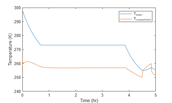
Both the ice compartment and water get colder for the first 40 minutes. The water reaches its freezing point around 40 minutes and both the ice compartment and water temperatures stay constant as the water freezes. After the water is completely freezes, the temperatures start to drop until the system turns off the compressor and fans. The refrigeration cycle turns on and off to keep the ice compartment at the temperature setpoint for the rest of the simulation.

Next, plot the phases of the water.

phase = simlog_IceMaker.Thermal_Network.Freezing_Water.internal_mode_var_mc1__.series.values;
plot(t_model, phase, 'LineWidth', 2);
ylim([0, 4]);
yticks([1, 2, 3]);
yticklabels({'Solid', 'Liquid', 'Solid <-> Liquid'});
xlabel('Time (hr)');
ylabel('Phase');

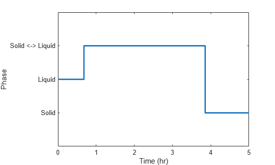
The freezing water block is in the liquid phase for approximately 40 minutes. The water then transitions between liquid and solid states before becoming solid. These phases and their timing are consistent with the discontinuous temperature changes in the freezing water block.