Tandem Primary Cylinder
R2026bThis example shows how to model, parameterize and test a tandem primary cylinder starting from manufacturer data sheet information. Given the numerical data extracted from the data sheet, the example uses optimization to determine remaining unknown parameters. After you run the model you can compare the resulting push rod force - brake pressure relationship curve with the curve provided on the manufacturer data sheet.
Model
The following figure shows the tandem primary cylinder test harness. Spring-loaded accumulators are used for loading in the and the circuits in place of disk or drum brakes. The input to the model is the push rod force coming from the lever mechanism or the brake booster. Output of the model is the pressures achieved in the brake circuits 1 and 2 respectively.
open_system('TandemPrimaryCylinder')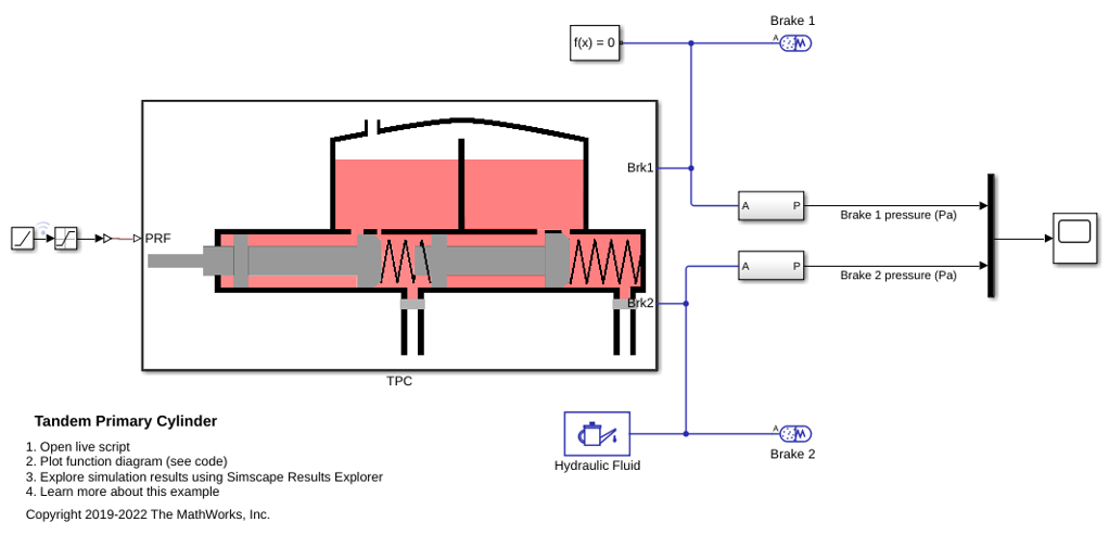
Manufacturer Data Sheet Data
The supplier data sheet includes the following data.
dp : first and second circuit piston diameter.
stroke1 : first circuit piston stroke.
stroke2 : second circuit piston stroke.
totalStroke : overall stroke.
disp1 : first circuit displacement.
disp2 : second circuit displacement.
totalDisp : net displacement.
maxPress : max pressure.
Load the data sheet. There are 4 available data sheets.
tpc.sheetNum = 1;
TandemPrimaryCylinderData
Pressure Development Characteristics
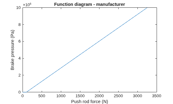
Plot the function diagram or the push rod force-brake pressure curve for the tandem primary cylinder.
p1 = plot(tpc.pushRodF,tpc.circuitP);
p2 = xlabel('Push rod force (N)');
p3 = ylabel('Brake pressure (Pa)');
p4 = title('Function diagram - manufacturer');
Equations of Motion (EoM) of System
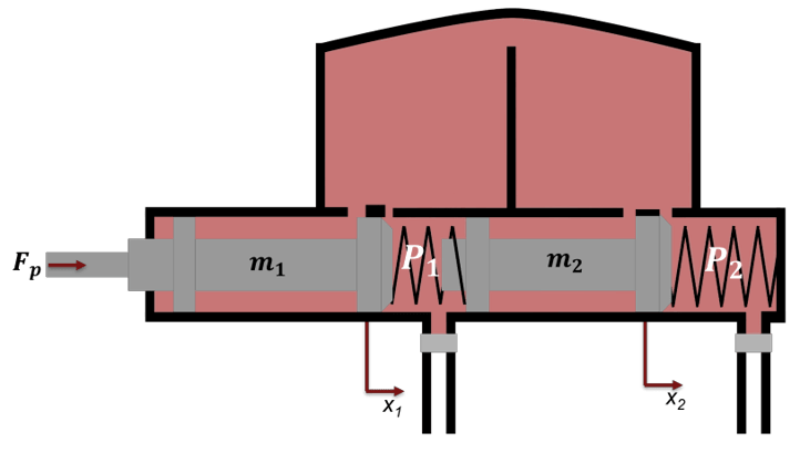
The following figure shows the tandem primary cylinder. Mass 1 and mass 2 use the coordinate frames shown below. This description only includes the mechanical EoM of the system and does not include the fluid dynamics equations.
, when
, when
, when
, when
where:
and are positions of piston mass 1 and mass 2 from the left side assumed hard stop.
and are masses of piston 1 and 2 respectively.
and are damping coefficients of piston 1 and 2 respectively.
and are stiffness coefficients of left (Spring 1) and right (spring 2) respectively.
is force applied on push rod of primary cylinder.
and are pressures in brake circuit 1 and 2 respectively.
and are reaction forces on mass 1 and 2 respectively when both masses are at the leftmost position.
and are preloads on left and right side springs respectively.
Parameter Estimation Method
Some parameters, which are important for functionality assessment, are not provided in the manufacturer's data sheet. To simulate the model you can estimate these parameters. Convert the EoM to steady state equations to estimate unknown parameters.
, when
, when
, when
, when
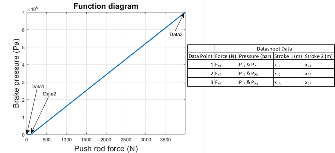
This figure shows data for the function diagram.
where:
and are the push rod forces for points 1,2, and 3 respectively.
,Here is for the brake circuit pressures at points 1,2, and 3 respectively.
and represent the leftmost positions for piston 1 and 2 respectively.
and as per the manufacturer data sheet data.
and are piston positions at data point 2. This point needs to be iterated on during optimization to estimate the unknown parameters.
The estimation scheme is:
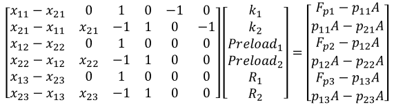
The estimation should yield results with the following conditions met:
and should be greater than or equal to 0.
and should be greater than 0.
Parameter Estimation Scheme
Define initial parameter values.
tpc.x11 = 0;                                      % (m)  opening length compensating port 1
tpc.x21 = 0;                                      % (m)  opening length compensating port 2

tpc.x12v = (0.5e-3:0.005e-3:1.5e-3);              % (m)  Assumed vector - user supplied to estimate x12
tpc.x22v = (0.5e-3:0.005e-3:1.5e-3);              % (m)  Assumed vector - user supplied to estimate x22

tpc.x13 = tpc.totalStroke;                        % (m)
tpc.x23 = tpc.stroke2;                            % (m)

tpc.fP1 = tpc.pushRodF(1);                        % N
tpc.fP2 = tpc.pushRodF(2);                        % N
tpc.fP3 = tpc.pushRodF(3);                        % N

tpc.p11 = tpc.circuitP(1);                        % N/m^2
tpc.p12 = tpc.circuitP(2);                        % N/m^2
tpc.p13 = tpc.circuitP(3);                        % N/m^2

tpc.p21 = tpc.p11;                                % N/m^2
tpc.p22 = tpc.p12;                                % N/m^2
tpc.p23 = tpc.p13;                                % N/m^2
tpc.aPist = (pi/4)*tpc.dp^2;                      % (m^2) Pressure acting piston area
Run the parameter estimation scheme.
tpc.x12size = size(tpc.x12v);
tpc.x22size = size(tpc.x22v);
tpc.checkPar = [];
for ii = 1:tpc.x12size(2)
    tpc.x12 = tpc.x12v(ii);
    for jj = 1:tpc.x22size(2)
        tpc.x22 = tpc.x22v(jj);
        tpc.a = [tpc.x11-tpc.x21     0    1  0 -1  0;...
            tpc.x21-tpc.x11 tpc.x21 -1  1  0 -1;...
            tpc.x12-tpc.x22     0    1  0  0  0;...
            tpc.x22-tpc.x12 tpc.x22 -1  1  0  0;...
            tpc.x13-tpc.x23     0    1  0  0  0;...
            tpc.x23-tpc.x13 tpc.x23 -1  1  0  0];

        tpc.b = [tpc.fP1-tpc.p11*tpc.aPist;...
            tpc.p11*tpc.aPist-tpc.p21*tpc.aPist;...
            tpc.fP2-tpc.p12*tpc.aPist;...
            tpc.p12*tpc.aPist-tpc.p22*tpc.aPist;...
            tpc.fP3-tpc.p13*tpc.aPist;...
            tpc.p13*tpc.aPist-tpc.p23*tpc.aPist];

        tpc.out = tpc.a\tpc.b;

        tpc.k1 = tpc.out(1);              % (N/m) First spring stiffness
        tpc.k2 = tpc.out(2);              % (N/m) Second spring stiffness
        tpc.preload1 = tpc.out(3);           % (N) First spring preload force
        tpc.preload2 = tpc.out(4);           % (N) Second spring preload force
        tpc.r1 = tpc.out(5);              % (N) Reaction on first mass at rest
        tpc.r2 = tpc.out(6);              % (N) Reaction on second mass at rest
        tpc.defLL = tpc.preload1/tpc.k1;     % (m) First spring compression
        tpc.defLR = (tpc.preload2)/tpc.k2;   % (m) First spring compression
        if tpc.r1>=0 && tpc.r2>=0 && tpc.preload2>=tpc.preload1 && tpc.k1>0 && tpc.k2>0
            tpc.checkPar = 1;
            break
        end
    end
    if tpc.r1>=0 && tpc.r2>=0 && tpc.preload2>=tpc.preload1 && tpc.k1>0 && tpc.k2>0 && tpc.checkPar==1
        tpc.k1 = tpc.out(1);              % (N/m) First spring stiffness
        tpc.k2 = tpc.out(2);              % (N/m) Second spring stiffness
        tpc.preload1 = tpc.out(3);           % (N) First spring preload force
        tpc.preload2 = tpc.out(4);           % (N) Second spring preload force
        tpc.r1 = tpc.out(5);              % (N) Reaction on first mass at rest
        tpc.r2 = tpc.out(6);              % (N) Reaction on second mass at rest
        tpc.defLL = tpc.preload1/tpc.k1;     % (m) First spring compression
        tpc.defLR = (tpc.preload2)/tpc.k2;   % (m) First spring compression
        tpc.x12 = tpc.x12;                % (m) Point as per section parameter estimation scheme
        tpc.x22 = tpc.x22;                % (m) Point as per section parameter estimation scheme
        fprintf(['Parameters K1, K2, Preload1, Preload2, R1, R2, DefLL, DefLR are as per \niteration performed on data sheet parameters' ...
            ' x12 and X22. Other \nsolutions are also possible for different values of x12 and x22.'])
        break
    elseif ii==tpc.x12size(2)
        error('Problem does not have a closed form solution or try again by changing range vector of x12 and x22.')
        exit %#ok
    end
end
Parameters K1, K2, Preload1, Preload2, R1, R2, DefLL, DefLR are as per
iteration performed on data sheet parameters x12 and X22. Other
solutions are also possible for different values of x12 and x22.
Note that x12 and x22 values estimated from the algorithm along with the assumed parameters affect the output of the system simulation predominantly in the frequency domain. This is an example of a system where if you only perform model fitting in the time domain, then there may be unrepresentative behavior in the frequency domain.
Set estimation conditions for physical limits on parameters.
if tpc.r1<0 || tpc.r2<0
    error('Preload forces must be greater than or equal to zero.')
    exit  %#ok
end
if tpc.k1<=0 || tpc.k2<=0
    error('Spring stiffness must be positive')
    exit  %#ok
end
Prepare Model for Simulation
Define additional parameters. Some of the following parameters can be estimated with assumptions.
tpc.c1 = 1e-3;                                          % (Ns/m) Damping coefficient for piston 1
tpc.c2 = 1e-3;                                          % (Ns/m) Damping coefficient for piston 2
tpc.mass1 = 1e-2;                                       % (Kg) Piston 1 mass
tpc.mass2 = 1e-2;                                       % (Kg) Piston 2 mass
tpc.v2D = 1000e-9;                                      % (m^3) Brake circuit 1 dead Volume
tpc.v2M = tpc.v2D+tpc.aPist*(tpc.x13-tpc.x23);          % (m^3) Brake circuit 1 max Volume
tpc.v4D = 1000e-9;                                      % (m^3) Brake circuit 2 dead Volume
tpc.v4M = tpc.v4D+tpc.aPist*(tpc.x23);                  % (m^3) Brake circuit 2 dead Volume
tpc.a1Ori = 100e-6;                                     % (m^2) Compensating orifice area
tpc.a2Ori = 10e-6;                                      % (m^2) Brake circuit orifice area
tpc.pRes = 1.01325e5;                                   % (Pa) Initial Pressure condition
tpc.hss = 1e8;                                          % (N/m) Hard stop stiffness
tpc.hsd = 1e6;                                          % (N/(m/s)) Hard stop damping coefficient
It is important to test the system with the correct load. In the test model, loading is done on the tandem primary cylinder using spring-based accumulators. The data sheet provides the stroke values for brake circuits 1 and 2. Iterated parameters and are important for deciding the fluid chamber capacity of the accumulators.
Define the load circuit parameters
tpc.vol1 = tpc.v2M-tpc.v2D-tpc.aPist*tpc.x12;        % (m^3) Fluid chamber capacity for brake circuit 1
tpc.vol2 = tpc.v4M-tpc.v4D-tpc.aPist*tpc.x22;        % (m^3) Fluid chamber capacity for brake circuit 2
tpc.loadP1 = tpc.circuitP(3);                        % (Pa) Pressure at full capacity for brake circuit 1
tpc.loadP2 = tpc.circuitP(3);                        % (Pa) Pressure at full capacity for brake circuit 2
Simulate the model and plot the results.
simT = (tpc.pushRodF(3)/25)+10; % Simulation time
sim('TandemPrimaryCylinder',simT)
TandemPrimaryCylinderPlotPCharacteristics;
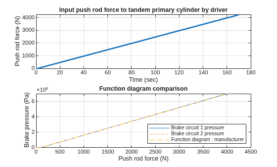
The model generates push rod force-brake pressure plots for selected manufacturer designs. The applied push rod force to the tandem primary cylinder is ramped at a 25 N/sec rate in the simulation.

