Poisson's Equation on Unit Disk: PDE Modeler App
This example shows how to solve the Poisson's equation on a unit disk and evaluate the numeric solution error.
This example uses the PDE Modeler app. For a programmatic workflow, see Poisson's Equation on Unit Disk. Because the app and the programmatic workflow use different meshers, they yield slightly different results.
The problem formulation is –Δu = 1 in Ω, u = 0 on ∂Ω, where Ω is the unit disk. The exact solution is
To solve this problem in the PDE Modeler app, follow these steps:
Open the PDE Modeler app by using the
pdeModelercommand.Display grid lines by selecting Options > Grid.
Align new shapes to the grid lines by selecting Options > Snap.
Draw a circle with the radius 1 and the center at (0,0). To do this, first click the
 button. Then right-click the origin and drag to draw a circle.
Right-clicking constrains the shape you draw so that it is a circle rather than an
ellipse. If the circle is not a perfect unit circle, double-click it. In the
resulting dialog box, specify the exact center location and radius of the
circle.
button. Then right-click the origin and drag to draw a circle.
Right-clicking constrains the shape you draw so that it is a circle rather than an
ellipse. If the circle is not a perfect unit circle, double-click it. In the
resulting dialog box, specify the exact center location and radius of the
circle.Check that the application mode is set to Generic Scalar.
Specify the boundary conditions. To do this, switch to boundary mode by clicking the
 button or selecting Boundary > Boundary Mode. Select all boundaries by selecting Edit > Select All. Then select Boundary > Specify Boundary Conditions and specify the Dirichlet boundary condition u = 0. This boundary condition is the default (
h = 1,r = 0), so you do not need to change it.Specify the coefficients by selecting PDE > PDE Specification or clicking the
 button on the toolbar. Specify
 c = 1,a = 0, andf = 1.Specify the maximum edge size for the mesh by selecting Mesh > Parameters. Set the maximum edge size to 0.1.
Initialize the mesh by selecting Mesh > Initialize Mesh or clicking the
 button.
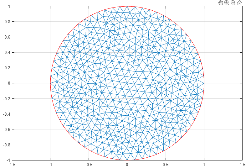
Solve the PDE by selecting Solve > Solve PDE or clicking the
 button on the toolbar. The toolbox assembles the
PDE problem, solves it, and plots the solution.
button on the toolbar. The toolbox assembles the
PDE problem, solves it, and plots the solution. 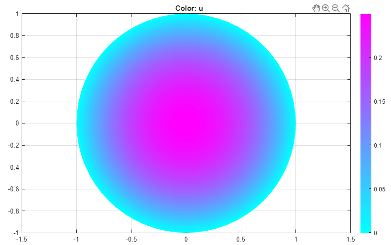
Compare the numerical solution to the exact solution:
Select Plot > Parameters.
In the resulting dialog box, select
user entryfrom the Color drop-down menu.Plot the absolute error in the solution by typing the MATLAB® expression
u-(1-x.^2-y.^2)/4in the User entry field.

Refine the mesh by selecting Mesh > Refine Mesh or clicking the
 button.
Compare the numerical solution to the exact solution for the refined mesh. Plot the absolute error.

Export the mesh data and the solution to the MATLAB workspace by selecting Mesh > Export Mesh and Solve > Export Solution, respectively.