CRLB for Bistatic Position Estimation

Since R2026a

This example demonstrates how to compute the Cramer-Rao lower bound (CRLB) for target position estimation in a 2D bistatic radar scenario. The CRLB provides a theoretical lower bound on the variance of unbiased estimators, offering insight into the best achievable accuracy for a given measurement model.

In this example, a single transmitter and receiver are placed at specified locations, and the CRLB is evaluated across a grid of target positions (the region of interest, ROI). The measurement model includes bistatic range and angle, each corrupted by independent Gaussian noise. The resulting CRLB is visualized to highlight regions of high and low estimation accuracy.

% ROI
x_ROI = -40:40; % m
y_ROI = -40:40; % m

% Bistatic transmitter and receiver positions
txpos = [-20.1;3.5]; % m
rxpos = [20.5;-1.2]; % m

Let $$p=[x;y]$$ be the target position, let $$p_{tx}$$ be the bistatic transmitter position, and let $$p_{rx}$$ be the bistatic receiver position. A bistatic measurement contains the following two pieces of information:

• Bistatic range: $$||p-p_{tx}||+||p-p_{rx}||-||p_{tx}-p_{rx}||$$.

• Angle from the target to the bistatic receiver: $${\tan }^{-1}\left(\frac{p(2)-p_{rx}(2)}{p(1)-p_{rx}(1)}\right)$$.

% Bistatic measurement model
measurement = @(tgtpos) [...
    % Bistatic range
    norm(tgtpos-txpos)+ norm(tgtpos-rxpos)- norm(txpos - rxpos);... % m
    % Angle from target to receiver
    atan2(tgtpos(2)-rxpos(2),tgtpos(1)-rxpos(1))]; % rad

The bistatic range measurement noise and angle measurement noise are independent. Thus, the measurement covariance matrix is a diagonal matrix with range measurement noise and angle measurement noise on the diagonal.

% Measurement covariance
range_noise = 1^2; % m^2
angle_noise = 0.2^2; % rad^2
measure_cov = diag([range_noise,angle_noise]);

The trace of the CRLB matrix sums the variances of the x and y position estimates, giving the total mean squared error (MSE) lower bound for 2D position estimation. Taking the square root of this sum yields the root mean squared error (RMSE) lower bound, which has the unit of meters—matching the units on the x- and y-axes of the visualization. Using RMSE in meters provides an intuitive, direct sense of the expected localization accuracy at each point in the ROI. By computing and plotting the square root of the CRLB across the ROI with the bistatic measurement model and measurement covariance, we can clearly visualize how position estimation accuracy varies spatially in terms of actual distance.

% Numerical square root of CRLB of 2-D bistatic position estimation
posest_sqrt_crlb = zeros(length(y_ROI),length(x_ROI));
for xidx = 1:length(x_ROI)
    for y_idx = 1:length(y_ROI)
        param = [x_ROI(xidx); y_ROI(y_idx)];
        
        crlb_matrix = crlb(measurement, measure_cov, param, DataComplexity = 'Real');
        posest_sqrt_crlb(y_idx,xidx) = sqrt(trace(crlb_matrix));
    end
end

Visualizing the square root of the CRLB across the ROI provides insight into the achievable accuracy of bistatic position estimation at different target locations. To enhance the visualization, the upper limit of the displayed color bar is set to 30. This is because, without setting an upper limit, a few extremely large square root of CRLB values would dominate the color scale, making it difficult to distinguish variations in the square root of the CRLB across most of the region, where values are typically smaller than 30.

% Display result
uplim = 30;
posest_sqrt_crlb(posest_sqrt_crlb > uplim) = uplim;
clims = [0,uplim];
imagesc([x_ROI(1),x_ROI(end)],[y_ROI(1),y_ROI(end)],posest_sqrt_crlb,clims)
hold on
plot(txpos(1,1),txpos(2,1),"v",...
    'MarkerSize',12,'MarkerEdgeColor','r','MarkerFaceColor',"k")
plot(rxpos(1,1),rxpos(2,1),"^",...
    'MarkerSize',12,'MarkerEdgeColor','g','MarkerFaceColor',"k")
cb = colorbar;
ylabel(cb, 'RMSE Lower Bound (m)');
xlabel('x (m)')
ylabel('y (m)')
legend('Transmitter','Receiver')

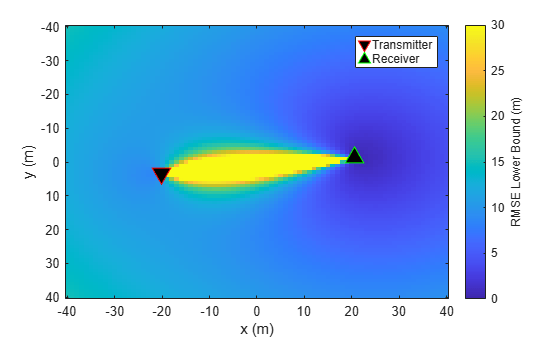
The above result shows that position estimation error is generally higher when the target is located near the baseline between the transmitter and receiver, illustrating a fundamental limitation in bistatic localization geometry. In addition, the CRLB is lower near the receiver because the angle measurement is referenced to the receiver’s position. This means that small changes in the target’s location produce larger changes in the measured angle when the target is close to the receiver, resulting in a sharper likelihood curvature in that region. Consequently, the localization accuracy improves (i.e., the CRLB is lower) near the receiver.