Direction of Arrival Estimation Using the Measured Array Manifold

Since R2026a

Introduction

There are many ways to model antenna array response patterns. Idealized, closed-form models are derived from array geometry; higher-fidelity models use numerical solvers of Maxwell’s equations. However, even the highest fidelity models can miss individual array-specific effects such as geometric perturbations. In high-precision direction-of-arrival (DOA) systems using super-resolution methods such as MUSIC, the array manifold is often measured directly. This example shows how to apply the MUSIC algorithm using a measured array manifold.

Background

The array manifold is a dictionary of values that maps the complex response at each antenna element to incident angle, frequency, and polarization of a plane wave arriving at the array. Typically, the manifold is obtained in an anechoic chamber by moving a calibrated transmit probe operating at a known frequency to discrete azimuth and elevation points and measuring the complex response at each antenna element. The following figure shows a measurement scheme and an example resultant array manifold as a table of measured values:

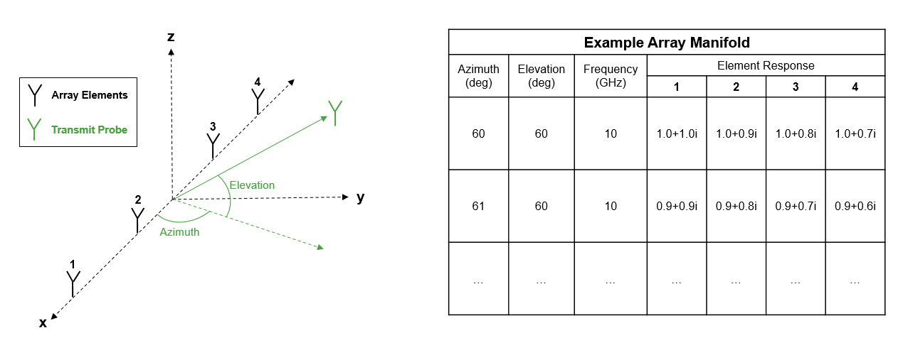
The array manifold is a high fidelity representation of the array response that captures effects such as mutual coupling and geometric perturbations.

Because we do not have access to a real measured array manifold in this example, we use the technique described in Comparison of Antenna Array Transmit and Receive Manifold (Antenna Toolbox) to generate a simulated version. This simulation approach captures effects not available in some lower fidelity models such as mutual coupling at the expense of increased computation times.

In this example, the pattern is simulated at a single frequency and single elevation with no polarization information so that it runs quickly. In practice, the manifold would likely span multiple frequencies, azimuths, elevations, and may include both vertical and horizontal polarization data.

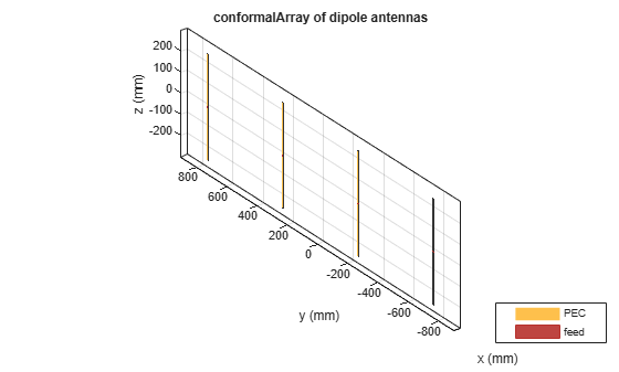
To generate a simulated manifold, we construct an array made up of dipole elements with half-wavelength spacing.

fc = 3e8;
lambda = freq2wavelen(fc);
M = 4;
antennapos = [zeros(1,M);(-(M-1)/2:(M-1)/2)*lambda/2;zeros(1,M)];
d = dipole(Length=lambda/2,Width=lambda/100);
array = conformalArray(Element=repmat(d,1,M),ElementPosition=antennapos');
figure;
show(array);

The manifold is simulated using the helperGenerateArrayManifold function. The output of this function is an object called a helperArrayManifold, which stores the simulated measurements.

fmeas = 3e8;
azmeas = -90:90;
elmeas = 0;
manifold = helperGenerateArrayManifold(array,fmeas,azmeas,elmeas);
disp(manifold);

  helperArrayManifold with properties:

     Manifold: [181×4 double]
    Frequency: [181×1 double]
      Azimuth: [181×1 double]
    Elevation: [181×1 double]

The main purpose of this object is to output the array response at a given angle and frequency.

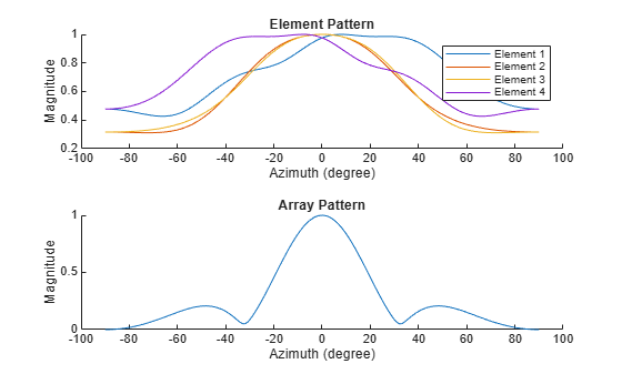
We can plot the normalized element patterns as well as the full array pattern using this helper object.

fplot = 3e8;
azplot = -90:90;
elplot = 0;
tl = tiledlayout(figure);
elax = nexttile(tl);
arrayax = nexttile(tl);
elementPattern(manifold,fplot,azplot,elplot,Parent=elax);
arrayPattern(manifold,fplot,azplot,elplot,Parent=arrayax);

This simulated manifold could be substituted with a real manifold measured in an anechoic chamber.

Signal Simulation

To demonstrate the workflow, we simulate signals impinging on the array using the same approach that was used to measure the array manifold. This makes the example internally consistent because both the manifold and the signals are derived from the same electromagnetic model.

In this example, we have two signals arriving from different directions.

% Number of samples in signal
nSamples = 1e5;

% Carrier frequency of both signals is 3e8
fc = 3e8;

% Signals are randomly generated
nSig = 2;
sig = randn(nSamples,nSig,like=1i);

% Angle of arrival
ang = [43 -12;0 0];

% Receiver used to add noise
rx = phased.Receiver(NoiseFigure=10);

% Collect received signal and add noise
sigcollect = helperCollectSignal(array,sig,fc,ang);
sigrx = rx(sigcollect);

In practice, you can replace the simulated snapshot with your recorded array data, and the processing remains unchanged. The simulation in this example is therefore a stand-in for your true data source.

Direction of Arrival Estimation

In this example the measured pattern is defined on an azimuth–elevation grid; in general, you may need to transform coordinates to match your processing frame and array orientation. This example uses a nearest neighbor approach for interpolation; depending on grid density and smoothness requirements, linear or higher-order interpolation methods may be preferable. We assume a narrowband model; for wideband operation, a standard approach is per-subband processing and coherent or incoherent combining.

In this example, we demonstrate how the measured array manifold can be used for direction of arrival estimation using the MUSIC algorithm.

MUSIC

MUSIC is a commonly used super-resolution DOA algorithm. For more information on the MUSIC algorithm, see MUSIC Super-Resolution DOA Estimation.

The effectiveness of the MUSIC algorithm relies heavily on having an accurate representation of the array response based on the true signal DOA, which is why measuring the true array manifold may be beneficial in high precision applications.

The first step in the MUSIC algorithm is generating the sample covariance matrix based on the signal collected in the prior section.

scov = cov(sigrx);

The next step is calculating the eigenvectors and eigenvalues of the sample covariance matrix.

[v,d] = eig(scov);
d = diag(d);

Noise eigenvectors correspond to the lowest magnitude eigenvalues. We assume knowledge of the number of signals present to retrieve the noise eigenvectors. Use the noise eigenvectors to generate the noise subspace.

[~,dIdx] = sort(d);
noiseIdx = dIdx(1:(M-nSig));
vNoise = v(:,noiseIdx);
noiseSubspace = vNoise*vNoise';

Once the noise subspace is calculated, we need to use information about the array manifold to generate the MUSIC pseudo-spectrum. We generate the steering vectors across a grid of azimuths and elevations to do so.

% Define the search space
azSearch = -90:90;
nAz = length(azSearch);
elSearch = 0;
nEl = length(elSearch);

% Initialize the pseudo-spectrum for the measured manifold
musicSpectrum = zeros(nAz,nEl);

% Calculate pseudo-spectrum across search space using the measured array
% manifold
for iAz = 1:nAz
    for iEl = 1:nEl
        % Calculate the steering vector from the array manifold
        azmeas = azSearch(iAz);
        elmeas = elSearch(iEl);
        sv = steeringVector(manifold,fc,azmeas,elmeas);

        % Generate the MUSIC pseudo-spectrum at the given az-el for the
        % measured antenna manifold
        musicSpectrum(iAz,iEl) = 1/(sv*noiseSubspace*sv');
    end
end

We can draw the MUSIC pseudo-spectrum alongside the signal DOA to demonstrate the effectiveness of this approach.

ax = axes(figure);
hold(ax,"on");
xline(ax,ang(1,1),LineStyle="--",DisplayName='Signal 1 DOA');
xline(ax,ang(1,2),LineStyle="--",DisplayName='Signal 2 DOA');
plot(ax,azSearch,mag2db(abs(musicSpectrum)),DisplayName="MUSIC Spectrum");
title(ax,'MUSIC Pseudo-Spectrum');
xlabel(ax,'Azimuth (degree)');
ylabel(ax,'Magnitude (dB)');
legend(ax,location="northwest");

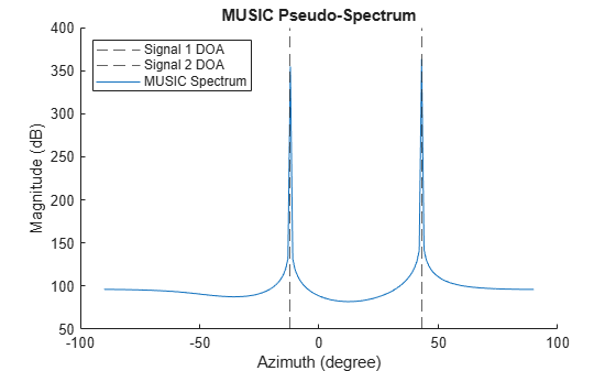
There are two sharp peaks clearly visible in the spectrum at the azimuth and elevation of the signals of interest. This demonstrates how you can perform DOA estimation using the MUSIC algorithm with a measured array manifold.

Conclusion

In this example we demonstrate how to implement a common DOA algorithm using a measured array manifold instead of an analytical model of an antenna array. This can be a very useful approach in cases when you do not have an adequate analytical model of your antenna array, but have data that was collected in a measurement chamber or calculated using a numerical solver.

References

[1] Friedlander, B. Antenna Array Manifolds for High-Resolution Direction Finding. IEEE Transactions on Signal Processing. 2017.

[2] Van Trees, H.L. Optimum Array Processing. New York, NY: Wiley-InterScience, 2002.

function manifold = helperGenerateArrayManifold(array,f,az,el)
    % Measure receive manifold from Comparison of Antenna Array Transmit and Receive Manifold

    % We measure response at each frequency, azimuth, and elevation
    nElements = length(array.Element);
    nFreq = length(f);
    nAzimuth = length(az);
    nElevation = length(el);
    nMeasurements = nAzimuth*nElevation*nFreq;

    % Initialize data storage
    azMeasurement = zeros(nMeasurements,1);
    elMeasurement = zeros(nMeasurements,1);
    freqMeasurement = zeros(nMeasurements,1);
    manifoldMeasurement = zeros(nAzimuth*nElevation*nFreq,nElements);

    % Setup the array elements
    nomLoad = lumpedElement(Impedance=[]);
    for m=1:nElements
        array.Element(m).Load = nomLoad;
    end

    % Calculate the response at each azimuth, elevation, and frequency
    idx = 1;
    for cAz = az
        for cEl = el
            for cFreq = f
                % Measure far field response
                erx = helperMeasureFarField(array,cAz,cEl,cFreq);

                % Save the measurement values
                azMeasurement(idx) = cAz;
                elMeasurement(idx) = cEl;
                freqMeasurement(idx) = cFreq;
                manifoldMeasurement(idx,:) = erx;

                idx = idx + 1;
            end
        end
    end

    manifold = helperArrayManifold(manifoldMeasurement,freqMeasurement,azMeasurement,elMeasurement);
end

function sigout = helperCollectSignal(array,sigin,f,ang)
    % Collect signal with carrier frequency f

    % Initialize data storage
    nElements = length(array.Element);
    nSample = size(sigin,1);
    nSigIn = size(sigin,2);

    % Initialize data storage
    sigout = zeros(nSample,nElements);

    % Setup the array elements
    nomLoad = lumpedElement(Impedance=[]);
    for m=1:nElements
        array.Element(m).Load = nomLoad;
    end
    
    % Calculate the reception of each signal
    for iSig = 1:nSigIn
        % Get current signal and angle of arrival
        cSig = sigin(:,iSig);
        cAz = ang(1,iSig);
        cEl = ang(2,iSig);

        erx = helperMeasureFarField(array,cAz,cEl,f);

        % Get the output signal
        sigout = sigout + erx.*cSig;
    end
end

function sv = helperMeasureFarField(array,az,el,f)
    % Calculate direction and polarization vector
    [x,y,z] = sph2cart(deg2rad(az),deg2rad(el),1);
    dirVec = [x;y;z];
    polVec = getPolVec(dirVec);
    
    % Measure the response
    p = planeWaveExcitation(Element=array,Direction=dirVec,Polarization=polVec);
    sv = feedCurrent(p,f);
end

function polVec = getPolVec(dirVec)
    % In this example, we calculate the polarization vector by projecting
    % the z unit vector onto the space orthogonal to the direction vector.
    % If the direction vector points in the z direction, set it to [1 0 0]
    % by default.
    k = [0;0;1];
    orthProj = k - dot(k,dirVec)/dot(dirVec,dirVec)*dirVec;
    if norm(orthProj) < sqrt(eps)
        polVec = [1;0;0];
    else
        polVec = orthProj / norm(orthProj);
    end
end