Vehicle Wheel Joint Configuration

R2026b

Compute wheel joint configuration for front-steered vehicle wheel spin visualization

Since R2026b

• 

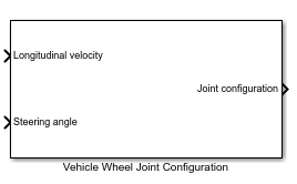
Vehicle Wheel Joint Configuration block

To add a block to a model, double-click the canvas and start typing the block name. Then, select the block from the list.

Libraries:
Offroad Autonomy Library / Vehicle Utilities

Description

The Vehicle Wheel Joint Configuration block computes the wheel joint configuration for front-steered vehicles.

The block assumes planar vehicle motion with pure rolling wheels (no longitudinal or lateral slip).

The block takes vehicle longitudinal velocity and steering angle as inputs and uses the vehicle's geometric parameters (wheel base, track widths, and wheel radii) to compute individual wheel angular velocities. The block integrates each angular velocity over time to determine the angular position of the wheel about its axle. The block then outputs these positions collectively as the wheel joint configuration. You can pass this output directly to a Simulation 3D Offroad Vehicle block to visualize wheel spin.

Use the Parameters tab to specify the vehicle geometry. Use the Wheel Body Mapping tab to specify the rigid body corresponding to each wheel joint.

This block does not require the Simulation 3D Scene Configuration block or Unreal Engine^® by itself. However, you can use these with the block in a model for full visualization of offroad applications.

Examples

Simulate Wheel Spin for Haul Truck

This example shows how to compute wheel joint configuration for a front-steered offroad vehicle using the Vehicle Wheel Joint Configuration block in Simulink®. You can use this joint configuration to visualize wheel spin in a 3-D simulation environment.

You can use the example to:

1. Load vehicle parameters from the offroad vehicle library.

2. Open and explore the Simulink model.

3. Simulate the model and visualize wheel spin.

4. Interpret the block outputs.

5. Compute per-wheel angular velocities.

Prerequisites

This example requires the Simulink 3D Animation™ with Unreal Engine® for full visualization.

To run only the wheel joint configuration computation, you can remove the Simulation 3D blocks and log the Vehicle Wheel Joint Configuration block output directly.

Load Vehicle Parameters

Load the haul truck rigid body tree model and vehicle geometry parameters from the offroad vehicle library. The loadvehicle function returns a rigidBodyTree object and a structure containing the wheel base, track width, and wheel radius.

[rbt, params] = loadvehicle("haultruck");
trackWidth = params.TrackWidth % in meters

trackWidth = 
7.3328

wheelBase = params.WheelBase % in meters

wheelBase = 
7.2593

wheelRadius = params.WheelRadius % in meters

wheelRadius = 
1.9747

initialState = [0 0 0 0]; % [x y theta psi]

The rigid body tree has five non-fixed joints: one bed pivot (for the truck bed) and four revolute wheel joints.

disp(rbt)

  rigidBodyTree with properties:

     NumBodies: 6
        Bodies: {[1×1 rigidBody]  [1×1 rigidBody]  [1×1 rigidBody]  [1×1 rigidBody]  [1×1 rigidBody]  [1×1 rigidBody]}
          Base: [1×1 rigidBody]
     BodyNames: {'body'  'bed_pivot'  'wheel_fl'  'wheel_fr'  'wheel_rl'  'wheel_rr'}
      BaseName: 'vehiclebody'
       Gravity: [0 0 -9.8100]
    DataFormat: 'struct'
    FrameNames: {'vehiclebody'  'body'  'bed_pivot'  'wheel_fl'  'wheel_fr'  'wheel_rl'  'wheel_rr'}

Open Simulink Model

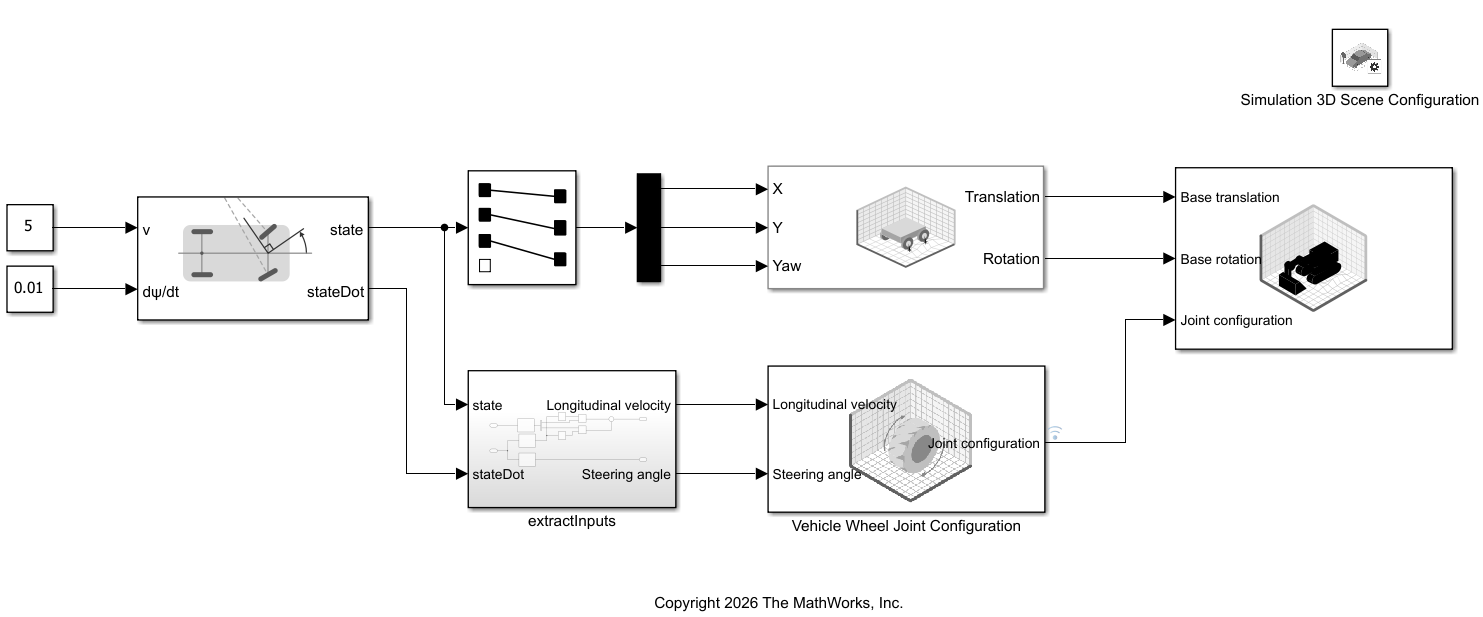
open_system("simulateHaulTruckWheelSpin");

The model simpleMotion_truck contains these key blocks:

• Constant1 (5) — Constant block representing a constant vehicle speed of 5 m/s

• Constant2 (0.01) — Constant block representing a constant steering angular velocity of 0.01 rad/s

• Ackermann Kinematic Model — Kinematic model block that computes vehicle motion using Ackermann steering geometry

• extractInputs — Subsystem block that extracts longitudinal velocity and steering angle from the kinematic model state and stateDot

• Vehicle Wheel Joint Configuration — Block that computes wheel angular positions from velocity and steering

• Simulation 3D Four-Wheel Ground Following — Block that computes terrain-aligned pose

• Simulation 3D Offroad Vehicle — Block that visualizes the haul truck vehicle in Unreal Engine

Simulate Model

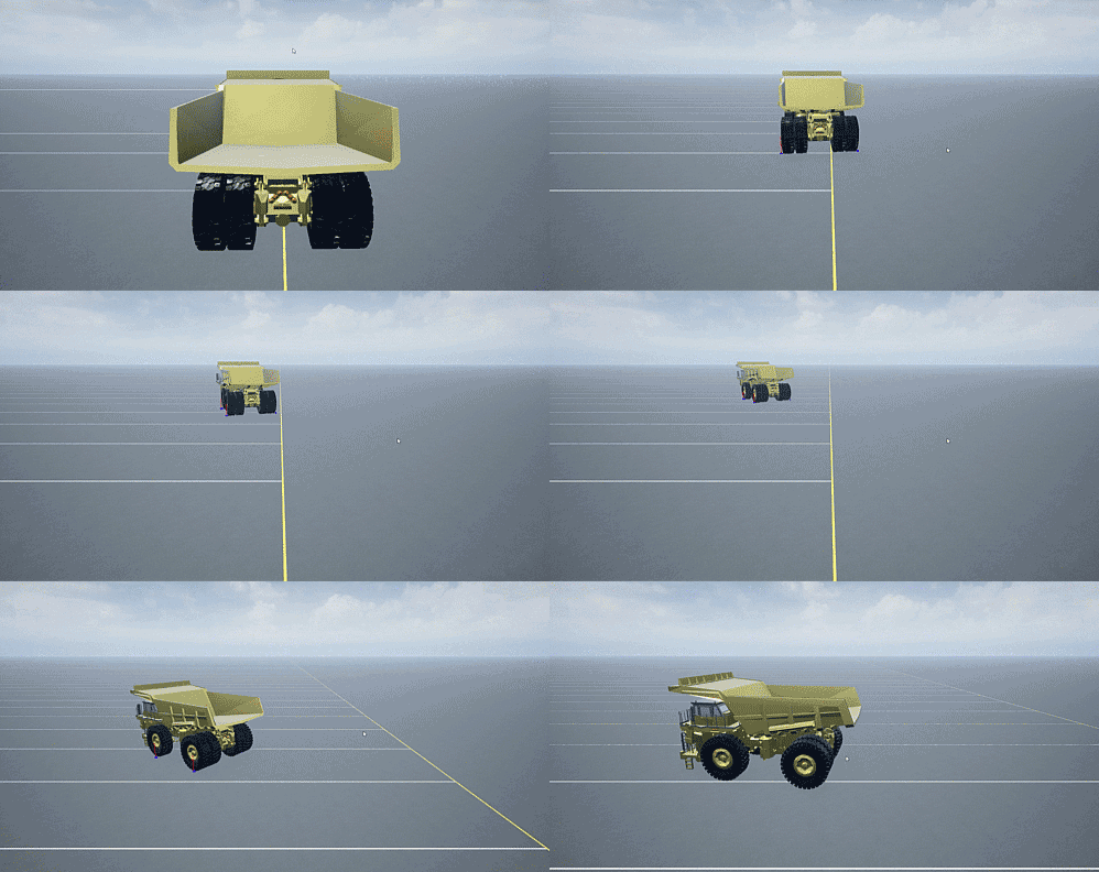
Simulate the model for 20 seconds. The Ackermann Kinematic Model drives the vehicle at 5 m/s with a constant steering angular velocity of 0.01 rad/s (gentle left turn), while the Vehicle Wheel Joint Configuration block computes the wheel angular positions at each time step. The Simulation 3D Offroad Vehicle block visualizes the haul truck in the 3-D simulation environment.

% Enable signal logging on Joint Configuration output of Vehicle Wheel Joint configuration block
ph = get_param("simulateHaulTruckWheelSpin/Vehicle Wheel Joint Configuration", "PortHandles");
set_param(ph.Outport(1), "DataLogging", "on", "DataLoggingName", "jointConfig");

% Run simulation
out = sim("simulateHaulTruckWheelSpin");

Visualize Wheel Spin of Vehicle

When you run this model, the Simulation 3D Offroad Vehicle block renders the haul truck in a 3-D environment with realistic wheel spin. The wheel joint configuration computed by the Vehicle Wheel Joint Configuration block drives the wheel rotation in the scene, enabling visual verification that the wheels spin at the correct differential rates during turns.

Interpret Block Outputs

The joint configuration output is a 5-by-1 vector at each time step. Each element corresponds to a non-fixed joint in the rigidBodyTree. You can inspect the joint order by calling rbt.homeConfiguration, which returns a 1-by-5 struct array. Understanding this order is essential for correctly filling out the wheel body mapping in the block.

For this model, index 1 is bed_pivot, indices 2–5 are wheel_fl, wheel_fr, wheel_rl, and wheel_rr.

Extract the logged joint configuration data.

jointConfig = out.jointConfig;
time = jointConfig.Time;
data = squeeze(jointConfig.Data);

%Ensure data is oriented as time-by-joints (rows are time steps, columns are joints).
%The squeeze function may return a transposed result depending on signal dimensions.

if size(data, 1) ~= length(time)
    data = data';
end

Verify that the bed pivot joint (index 1) remains zero throughout the simulation.

% Maximum absolute bed_pivot position (expected: 0)
maxBedPivotPosition = max(abs(data(:,1)))

maxBedPivotPosition = 
0

Compute Per-Wheel Angular Velocities

Compute per-wheel angular velocities by differentiating the angular positions.

The inner wheels (left, during a left turn) spin slower than the outer wheels (right) because they trace a shorter arc around the instantaneous center of rotation (ICR).

dt = diff(time);
omegaFL = diff(data(:,2)) ./ dt;
omegaFR = diff(data(:,3)) ./ dt;
omegaRL = diff(data(:,4)) ./ dt;
omegaRR = diff(data(:,5)) ./ dt;
timeMid = time(1:end-1) + dt/2;

Plot per-wheel angular velocities.

figure("Position", [100, 100, 900, 500])
subplot(2,1,1)
plot(timeMid, omegaFL, "b-", timeMid, omegaFR, "r-", "LineWidth", 1.5)
xlabel("Time (s)")
ylabel("\omega (rad/s)")
title("Front Wheel Angular Velocities")
legend("Front Left (inner)", "Front Right (outer)")
grid on

subplot(2,1,2)
plot(timeMid, omegaRL, "b-", timeMid, omegaRR, "r-", "LineWidth", 1.5)
xlabel("Time (s)")
ylabel("\omega (rad/s)")
title("Rear Wheel Angular Velocities")
legend("Rear Left (inner)", "Rear Right (outer)")
grid on

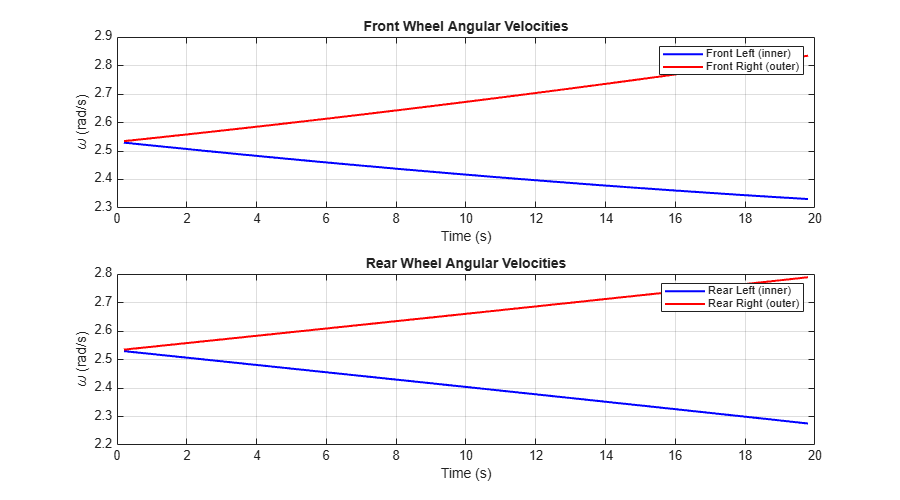
The plots show that the outer wheels (right side) spin faster than the inner wheels (left side) during the left turn. This differential is the Ackermann steering effect computed by the block using ICR kinematics.

Compute and display the mean angular velocities and the differential between inner and outer wheels.

meanOmegaFL = mean(omegaFL)

meanOmegaFL = 
2.4217

meanOmegaFR = mean(omegaFR)

meanOmegaFR = 
2.6766

meanOmegaRL = mean(omegaRL)

meanOmegaRL = 
2.4033

meanOmegaRR = mean(omegaRR)

meanOmegaRR = 
2.6608

differentialFront = meanOmegaFR - meanOmegaFL

differentialFront = 
0.2549

differentialRear = meanOmegaRR - meanOmegaRL

differentialRear = 
0.2575

Limitations

• The block assumes pure rolling, with no longitudinal or lateral slip.

• The block assumes planar vehicle motion.

• The block supports only front-steered vehicles. It does not support skid-steered, differential-drive, or articulated-steering vehicles, or vehicles with more than two axles.

• The block does not handle steering visualization (front wheel yaw rotation).

Ports

Input

Longitudinal velocity — Longitudinal velocity of vehicle

scalar

Longitudinal velocity of the vehicle, specified as a scalar in meters per second (m/s).

This input is the forward speed of the vehicle along its longitudinal axis.

Data Types: single | double

Steering angle — Front wheel steering angle

scalar

Front wheel steering angle, specified as a scalar in radians (rad).

This input is the steering angle of the front axle.

Data Types: single | double

Output

Joint configuration — Joint configuration vector containing wheel angular positions

vector

Joint configuration vector with wheel angular positions mapped to the corresponding rigid body joints, returned as an N-by-1 vector, where N is the number of non-fixed joints in the configured rigidBodyTree. The vector has a position for every non-fixed joint. Positions corresponding to joints that are not mapped to wheels are zero.

Because joints not mapped to wheels are zero, you can combine this output with joint configuration vectors from other modules (for example, a bucket arm controller) by using a Sum block. This configuration enables visualization of complete multi-joint vehicles.

Note

If there is a size mismatch between this output and the downstream Simulation 3D vehicle block, verify that both blocks use the same rigidBodyTree.

Data Types: single | double

Parameters

To edit block parameters interactively, use the Property Inspector. From the Simulink^® Toolstrip, on the Simulation tab, in the Prepare gallery, select Property Inspector.

Parameters

Wheel base (m) — Distance between front and rear axles

7.3 (default)

Distance between the front and rear axles of the vehicle, specified as a positive scalar in meters.

The block returns an error if you specify a value of zero or less.

Track width (m) — Distance between left and right wheels

7.3 (default)

Distance between the left and right wheels, specified as a positive scalar or a 1-by-2 vector in meters.

If you specify a scalar, the block uses the same track width for the front and rear axles. If you specify a 1-by-2 vector, the block interprets the values as [front axle track width, rear axle track width]. Use a vector if the vehicle has different front and rear track widths (for example, tractors).

The block returns an error if you specify a value of zero or less.

Wheel radius (m) — Radius of vehicle wheels

2 (default)

Radius of the vehicle wheels, specified as a positive scalar or a 1-by-2 vector in meters.

If you specify a scalar, the block uses the same radius for all wheels. If you specify a 1-by-2 vector, the block interprets the values as [front axle wheel radius, rear axle wheel radius]. Use a vector when the vehicle has different front and rear wheel sizes (for example, tractors).

The block returns an error if you specify a value of zero or less.

Wheel Body Mapping

Note

Verify that each wheel body parameter maps to the correct wheel position (front left to front left, front right to front right, and so on). Incorrect mapping causes wheels to spin at wrong speeds during simulation.

Rigid body tree — Rigid body tree model of vehicle

loadvehicle("haultruck") (default)

Rigid body tree model of the vehicle, specified as a rigidBodyTree object in the MATLAB workspace. The block uses this model to determine the number of non-fixed joints (which sets the joint configuration vector size) and the mapping from wheel angular positions to the correct joint indices.

Front left wheel body — Rigid body corresponding to front left wheel

vehiclebody (default)

Rigid body corresponding to the front left wheel, selected from the rigid body tree. The drop-down list shows only bodies with revolute joints.

Tip

If your wheel body does not appear in the drop-down list, verify that it uses a revolute joint in the rigidBodyTree.

Front right wheel body — Rigid body corresponding to front right wheel

vehiclebody (default)

Rigid body corresponding to the front right wheel, selected from the rigid body tree. The drop-down list shows only bodies with revolute joints.

Tip

If your wheel body does not appear in the drop-down list, verify that it uses a revolute joint in the rigidBodyTree.

Rear left wheel body — Rigid body corresponding to rear left wheel

vehiclebody (default)

Rigid body corresponding to the rear left wheel, selected from the rigid body tree. The drop-down list shows only bodies with revolute joints.

Tip

If your wheel body does not appear in the drop-down list, verify that it uses a revolute joint in the rigidBodyTree.

Rear right wheel body — Rigid body corresponding to rear right wheel

vehiclebody (default)

Rigid body corresponding to the rear right wheel, selected from the rigid body tree. The drop-down list shows only bodies with revolute joints.

Tip

If your wheel body does not appear in the drop-down list, verify that it uses a revolute joint in the rigidBodyTree.

Enable additional wheel bodies — Option to enable mapping for dual rear wheel bodies

off (default) | on

Select this parameter to enable additional rear wheel body mapping for vehicles with dual rear tires (for example, haul trucks). When you enable this paramter, the block assigns the same angular velocity as the corresponding rear wheel to the additional wheel body.

Selecting this parameter enables the Rear left additional wheel body and Rear right additional wheel body parameters.

Rear left additional wheel body — Rigid body corresponding to additional rear left wheel

''

Rigid body corresponding to the additional rear left wheel (for dual tire configurations), selected from the rigid body tree. The block assigns the same angular velocity as the rear left wheel to this body.

Dependencies

To enable this parameter, select Enable additional wheel bodies.

Rear right additional wheel body — Rigid body corresponding to additional rear right wheel

''

Rigid body corresponding to the additional rear right wheel (for dual tire configurations), selected from the rigid body tree. The block assigns the same angular velocity as the rear right wheel to this body.

Dependencies

To enable this parameter, select Enable additional wheel bodies.

Simulate using — Type of simulation to run

Interpreted execution (default) | Code generation

Specify the type of simulation to run.

• Code generation — Simulate model using generated C code. The first time you run a simulation, Simulink generates C code for the block. Subsequent simulations reuse the C code, as long as the model does not change.

• Interpreted execution — Simulate model using the MATLAB^® interpreter. For more information, see Interpreted Execution vs. Code Generation (Simulink).

Tunable: No

Algorithms

Wheel Angular Velocity from ICR Kinematics

The block uses the instantaneous center of rotation (ICR) to compute individual wheel angular velocities from the longitudinal velocity and steering angle of the vehicle.

This diagram represents the Ackermann steering geometry of a front-steered vehicle, showing the ICR and the geometric parameters that the algorithm uses to compute individual wheel angular velocities.

The following equations that describe block behavior use these variables:

• L is the wheel base.

• Tf is the front track width.

• Tr is the rear track width.

• Rf is the front wheel radius.

• Rr is the rear wheel radius.

• vx is the longitudinal velocity.

• ψ is the steering angle.

• ω is the angular velocity.

Straight-Line Motion

When |tan(ψ)| < 10⁻³, the block treats motion as straight-line and assigns equal angular velocities to all wheels on each axle:

ωFl = ωFr = vx / Rf
ωRl = ωRr = vx / Rr

where ωFl and ωFr are the front left and front right wheel angular velocities, and ωRl and ωRr are the rear left and rear right wheel angular velocities.

Turning Motion

When |tan(ψ)| ≥ 10⁻³, the block uses Ackermann steering geometry to compute the individual wheel angular velocities.

The block first computes the turning radius R, which is the distance from the ICR to the center of the rear axle:

R = L / tan(ψ)

The block then computes the vehicle yaw rate:

ω = vx / R

Using the yaw rate and the distance of each wheel from the ICR, the block computes the individual wheel angular velocities:

ωRl = ω × (R - Tr/2) / Rr
ωRr = ω × (R + Tr/2) / Rr
ωFl = ω × sqrt((R - Tf/2)² + L²) / Rf
ωFr = ω × sqrt((R + Tf/2)² + L²) / Rf

Integration for Wheel Joint Position

The block integrates each wheel angular velocity over time to determine the angular position of the wheel about its axle:

θ_wheel(t) = ∫ ω_wheel dt

The block assigns each computed wheel angular position to the corresponding joint in the rigidBodyTree using the mapping specified in the Wheel Body Mapping tab. Each wheel in the rigidBodyTree must use a revolute joint.

Version History

Introduced in R2026b