OptimResults

Estimation results object for any supported algorithm except nlinfit

Description

The OptimResults object contains estimation results from fitting a SimBiology^® model to data using the sbiofit function with any supported algorithm except nlinfit. See the sbiofit function for a list of supported algorithms.

Creation

Use sbiofit with any supported estimation algorithm except nlinfit to create an OptimResults object.

Properties

GroupName — Name of the group associated with the results

categorical | empty array

Name of the group associated with the results, specified as a categorical. If the 'Pooled' name-value pair argument was set to true when you ran sbiofit, then GroupName is returned as an empty array or [].

Beta — Table of estimated parameters

table

Table of estimated parameters, specified as a table. The jth row of the table represents the jth estimated parameter β_j. It contains transformed values of parameter estimates if any parameter transform is specified. Standard errors of these parameter estimates (StandardError) are calculated as: sqrt(diag(COVB)).

It can also contain the following variables:

• Bounds — the values of transformed parameter bounds that you specified during fitting

• CategoryVariableName — the names of categories or groups that you specified during fitting

• CategoryValue — the values of category variables specified by CategoryVariableName

This table contains one row per distinct parameter value.

ParameterEstimates — Table of estimated parameters

table

Table of estimated parameters, specified as a table. The jth row of the table represents the jth estimated parameter β_j. This table contains untransformed values of parameter estimates. Standard errors of these parameter estimates (StandardError) are calculated as: sqrt(diag(CovarianceMatrix)).

It can also contain the following variables:

• Bounds — the values of transformed parameter bounds that you specified during fitting

• CategoryVariableName — the names of categories or groups that you specified during fitting

• CategoryValue — the values of category variables specified by CategoryVariableName

This table contains sets of parameter values that are identified for each individual or group.

J — Jacobian matrix of the model

array

Jacobian matrix of the model, specified as an array. The Jacobian matrix with respect to an estimated parameter is

$$J(i,j,k)={\frac{\partial y_k}{\partial {\beta }_j}|}_{t_i}$$

where t_i is the ith time point, β_j is the jth estimated parameter in the transformed space, and y_k is the kth response in the group of data.

COVB — Estimated covariance matrix for Beta

matrix

Estimated covariance matrix for Beta, specified as a matrix. This matrix is calculated as: COVB = inv(J'*J)*MSE.

CovarianceMatrix — Estimated covariance matrix for ParameterEstimates

matrix

Estimated covariance matrix for ParameterEstimates, specified as a matrix. This matrix is calculated as: CovarianceMatrix = T'*COVB*T, where T = diag(JInvT(Beta)). JInvT(Beta) returns a Jacobian matrix of Beta which is inverse transformed accordingly if you specified any transform to estimated parameters.

For instance, suppose you specified the log-transform for an estimated parameter x when you ran sbiofit. The inverse transform is: InvT = exp(x), and its Jacobian is: JInvT = exp(x) since the derivative of exp is also exp.

R — Residuals matrix

matrix

Residuals matrix, specified as a matrix. R_ij is the residual for the ith time point and the jth response in the group of data.

LogLikelihood — Maximized loglikelihood for the fitted model

scalar

Maximized loglikelihood for the fitted model, specified as a scalar.

AIC — Akaike Information Criterion (AIC)

scalar

Akaike Information Criterion (AIC), specified as a scalar. The AIC is calculated as AIC = 2*(-LogLikelihood + P), where P is the number of parameters.

BIC — Bayes Information Criterion (BIC)

scalar

Bayes Information Criterion (BIC), specified as a scalar. The BIC is calculated as BIC = -2*LogLikelihood + P*log(N), where N is the number of observations, and P is the number of parameters.

DFE — Degrees of freedom for error

scalar

Degrees of freedom for error (DFE), specified as a scalar. The DFE is calculated as DFE = N-P, where N is the number of observations and P is the number of parameters.

MSE — Mean squared error

scalar

Mean squared error, specified as a scalar.

SSE — Sum of squared (weighted) errors or residuals

scalar

Sum of squared (weighted) errors or residuals, specified as a scalar.

Weights — Matrix of weights

matrix

Matrix of weights, specified as a matrix with one column per response and one row per observation.

Data — Data used for fitting

groupedData object

Data used for fitting, specified as a groupedData object.

In most cases, this Data property contains a copy of groupedData specified as the input data in the sbiofit call or the Data property of a fitproblem object. One exception is that the Data property of unpooled fit results objects contain only the subset of data for the individual group used for fitting.

EstimatedParameterNames — Estimated parameter names

cell array of character vectors

Estimated parameter names, specified as a cell array of character vectors.

ErrorModelInfo — Error models and estimated error model parameters

table

Error models and estimated error model parameters, specified as a table.

• The table has one row per error model.

• The ErrorModelInfo.Properties.RowsNames property identifies which responses the row applies to.

• The table contains three variables: ErrorModel, a, and b. The ErrorModel variable is categorical. The variables a and b can be NaN when they do not apply to a particular error model.

There are four built-in error models. Each model defines the error using a standard mean-zero and unit-variance (Gaussian) variable e, the function value f, and one or two parameters a and b. In SimBiology, the function f represents simulation results from a SimBiology model.

• 'constant': $$y=f+ae$$

• 'proportional': $$y=f+b\left|f\right|e$$

• 'combined': $$y=f+(a+b\left|f\right|)e$$

• 'exponential': $$y=f\ast \exp (ae)$$

EstimationFunction — Name of the estimation function

character vector

Name of the estimation function, specified as a character vector.

DependentFiles — File names to include for deployment

cell array of character vectors

File names to include for deployment, specified as a cell array of character vectors.

ExitFlag — Exit flag specific to the estimation function

scalar

Exit flag specific to the estimation function, specified as a scalar. See the reference page of the specific algorithm to get more information on the value of ExitFlag.

Output — Additional outputs specific to the estimation function

structure array

Additional outputs specific to the estimation function, specified as a structure array. See the reference page of the specific algorithm to get more information on the values of the Output structure array.

Object Functions

boxplot	Create box plot showing the variation of estimated SimBiology model parameters
fitted	Return simulation results of SimBiology model fitted using least-squares regression
plot	Compare simulation results to the training data, creating a time-course subplot for each group
plotActualVersusPredicted	Compare predictions to actual data, creating a subplot for each response
plotResidualDistribution	Plot the distribution of the residuals
plotResiduals	Plot residuals for each response, using time, group, or prediction as x-axis
predict	Simulate and evaluate fitted SimBiology model
random	Simulate SimBiology model, adding variations by sampling error model
summary	Return structure array that contains estimated values and fit quality statistics

Examples

Fit One-Compartment Model to Individual PK Profile

Background

This example shows how to fit an individual's PK profile data to one-compartment model and estimate pharmacokinetic parameters.

Suppose you have drug plasma concentration data from an individual and want to estimate the volume of the central compartment and the clearance. Assume the drug concentration versus the time profile follows the monoexponential decline $$C_t=C_0{e}^{-k_{e}t}$$, where $$C_t$$ is the drug concentration at time t, $$C_0$$ is the initial concentration, and $$k_e$$ is the elimination rate constant that depends on the clearance and volume of the central compartment $$k_e=Cl/V$$.

The synthetic data in this example was generated using the following model, parameters, and dose:

• One-compartment model with bolus dosing and first-order elimination

• Volume of the central compartment (Central) = 1.70 liter

• Clearance parameter (Cl_Central) = 0.55 liter/hour

• Constant error model

• Bolus dose of 10 mg

Load Data and Visualize

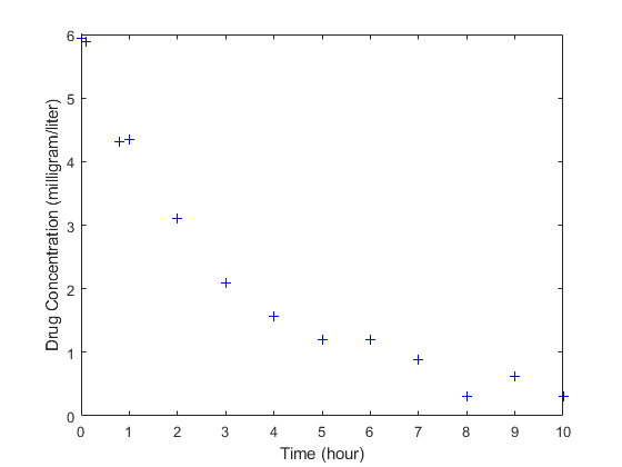
The data is stored as a table with variables Time and Conc that represent the time course of the plasma concentration of an individual after an intravenous bolus administration measured at 13 different time points. The variable units for Time and Conc are hour and milligram/liter, respectively.

load('data15.mat')
plot(data.Time,data.Conc,'b+')
xlabel('Time (hour)');
ylabel('Drug Concentration (milligram/liter)');

Convert to groupedData Format

Convert the data set to a groupedData object, which is the required data format for the fitting function sbiofit for later use. A groupedData object also lets you set independent variable and group variable names (if they exist). Set the units of the Time and Conc variables. The units are optional and only required for the UnitConversion feature, which automatically converts matching physical quantities to one consistent unit system.

gData = groupedData(data);
gData.Properties.VariableUnits = {'hour','milligram/liter'};
gData.Properties

ans = struct with fields:
                Description: ''
                   UserData: []
             DimensionNames: {'Row'  'Variables'}
              VariableNames: {'Time'  'Conc'}
              VariableTypes: ["double"    "double"]
       VariableDescriptions: {}
              VariableUnits: {'hour'  'milligram/liter'}
         VariableContinuity: []
                   RowNames: {}
           CustomProperties: [1×1 matlab.tabular.CustomProperties]
          GroupVariableName: ''
    IndependentVariableName: 'Time'

groupedData automatically set the name of the IndependentVariableName property to the Time variable of the data.

Construct a One-Compartment Model

Use the built-in PK library to construct a one-compartment model with bolus dosing and first-order elimination where the elimination rate depends on the clearance and volume of the central compartment. Use the configset object to turn on unit conversion.

pkmd                    = PKModelDesign;
pkc1                    = addCompartment(pkmd,'Central');
pkc1.DosingType         = 'Bolus';
pkc1.EliminationType    = 'linear-clearance';
pkc1.HasResponseVariable = true;
model                   = construct(pkmd);
configset               = getconfigset(model);
configset.CompileOptions.UnitConversion = true;

For details on creating compartmental PK models using the SimBiology® built-in library, see Create Pharmacokinetic Models.

Define Dosing

Define a single bolus dose of 10 milligram given at time = 0. For details on setting up different dosing schedules, see Doses in SimBiology Models.

dose                = sbiodose('dose');
dose.TargetName     = 'Drug_Central';
dose.StartTime      = 0;
dose.Amount         = 10;
dose.AmountUnits    = 'milligram';
dose.TimeUnits      = 'hour';

Map Response Data to the Corresponding Model Component

The data contains drug concentration data stored in the Conc variable. This data corresponds to the Drug_Central species in the model. Therefore, map the data to Drug_Central as follows.

responseMap = {'Drug_Central = Conc'};

Specify Parameters to Estimate

The parameters to fit in this model are the volume of the central compartment (Central) and the clearance rate (Cl_Central). In this case, specify log-transformation for these biological parameters since they are constrained to be positive. The estimatedInfo object lets you specify parameter transforms, initial values, and parameter bounds if needed.

paramsToEstimate    = {'log(Central)','log(Cl_Central)'};
estimatedParams     = estimatedInfo(paramsToEstimate,'InitialValue',[1 1],'Bounds',[1 5;0.5 2]);

Estimate Parameters

Now that you have defined one-compartment model, data to fit, mapped response data, parameters to estimate, and dosing, use sbiofit to estimate parameters. The default estimation function that sbiofit uses will change depending on which toolboxes are available. To see which function was used during fitting, check the EstimationFunction property of the corresponding results object.

fitConst = sbiofit(model,gData,responseMap,estimatedParams,dose);

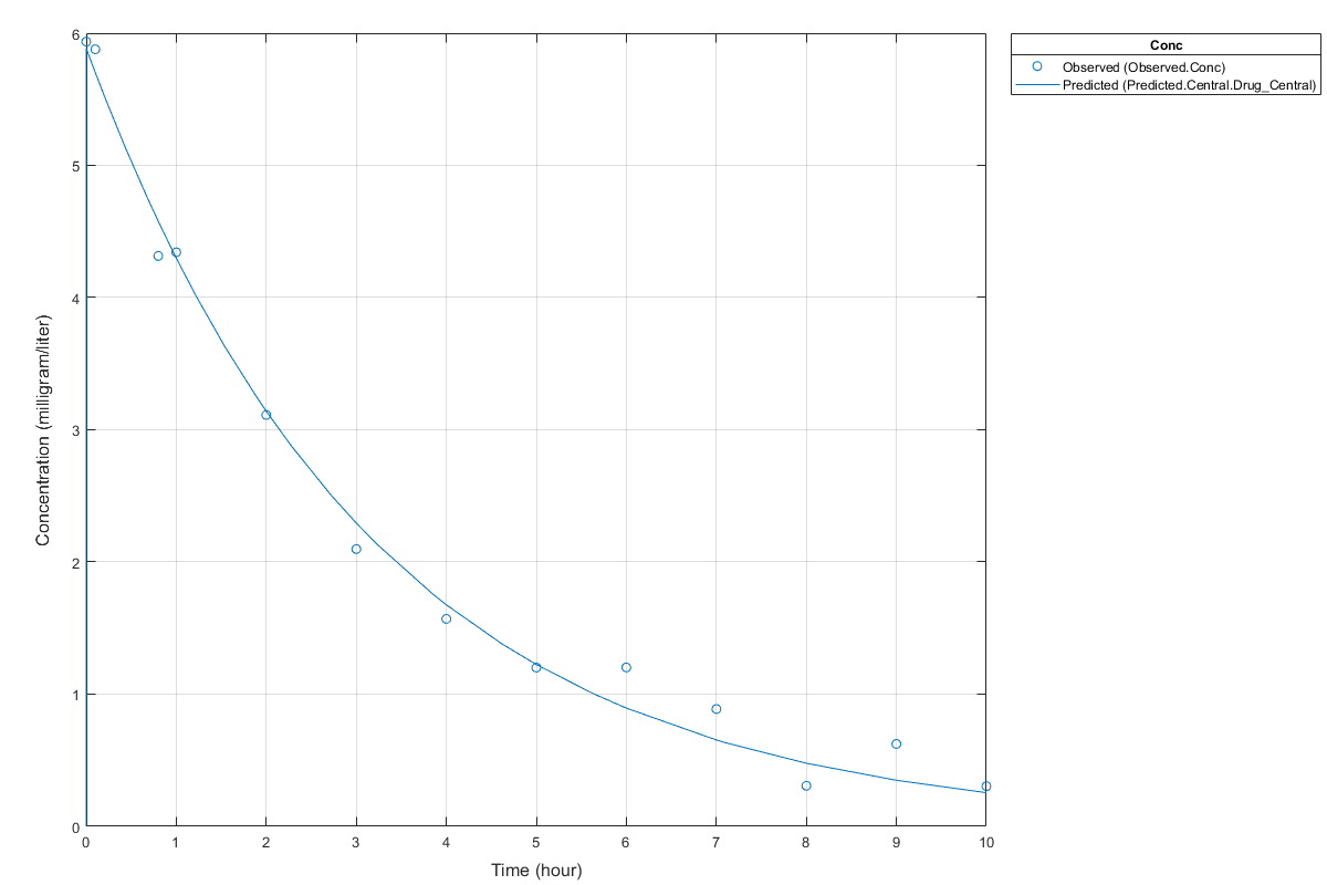
Display Estimated Parameters and Plot Results

Notice the parameter estimates were not far off from the true values (1.70 and 0.55) that were used to generate the data. You may also try different error models to see if they could further improve the parameter estimates.

fitConst.ParameterEstimates

ans=2×4 table
         Name         Estimate    StandardError      Bounds  
    ______________    ________    _____________    __________

    {'Central'   }     1.6993       0.034821         1      5
    {'Cl_Central'}    0.53358        0.01968       0.5      2

s.Labels.XLabel     = 'Time (hour)';
s.Labels.YLabel     = 'Concentration (milligram/liter)';
plot(fitConst,'AxesStyle',s);

Use Different Error Models

Try three other supported error models (proportional, combination of constant and proportional error models, and exponential).

fitProp = sbiofit(model,gData,responseMap,estimatedParams,dose,...
                      'ErrorModel','proportional');
fitExp  = sbiofit(model,gData,responseMap,estimatedParams,dose,...
                      'ErrorModel','exponential');
fitComb = sbiofit(model,gData,responseMap,estimatedParams,dose,...
                      'ErrorModel','combined');

Use Weights Instead of an Error Model

You can specify weights as a numeric matrix, where the number of columns corresponds to the number of responses. Setting all weights to 1 is equivalent to the constant error model.

weightsNumeric = ones(size(gData.Conc));
fitWeightsNumeric = sbiofit(model,gData,responseMap,estimatedParams,dose,'Weights',weightsNumeric);

Alternatively, you can use a function handle that accepts a vector of predicted response values and returns a vector of weights. In this example, use a function handle that is equivalent to the proportional error model.

weightsFunction = @(y) 1./y.^2;
fitWeightsFunction = sbiofit(model,gData,responseMap,estimatedParams,dose,'Weights',weightsFunction);

Compare Information Criteria for Model Selection

Compare the loglikelihood, AIC, and BIC values of each model to see which error model best fits the data. A larger likelihood value indicates the corresponding model fits the model better. For AIC and BIC, the smaller values are better.

allResults = [fitConst,fitWeightsNumeric,fitWeightsFunction,fitProp,fitExp,fitComb];
errorModelNames = {'constant error model','equal weights','proportional weights', ...
                   'proportional error model','exponential error model',...
                   'combined error model'};
LogLikelihood = [allResults.LogLikelihood]';
AIC = [allResults.AIC]';
BIC = [allResults.BIC]';
t = table(LogLikelihood,AIC,BIC);
t.Properties.RowNames = errorModelNames;
t

t=6×3 table
                                LogLikelihood      AIC        BIC  
                                _____________    _______    _______

    constant error model            3.9866       -3.9732    -2.8433
    equal weights                   3.9866       -3.9732    -2.8433
    proportional weights           -3.8472        11.694     12.824
    proportional error model       -3.8257        11.651     12.781
    exponential error model         1.1984        1.6032     2.7331
    combined error model            3.9163       -3.8326    -2.7027

Based on the information criteria, the constant error model (or equal weights) fits the data best since it has the largest loglikelihood value and the smallest AIC and BIC.

Display Estimated Parameter Values

Show the estimated parameter values of each model.

Estimated_Central       = zeros(6,1);
Estimated_Cl_Central    = zeros(6,1);
t2 = table(Estimated_Central,Estimated_Cl_Central);
t2.Properties.RowNames = errorModelNames;
for i = 1:height(t2)
    t2{i,1} = allResults(i).ParameterEstimates.Estimate(1);
    t2{i,2} = allResults(i).ParameterEstimates.Estimate(2);
end
t2

t2=6×2 table
                                Estimated_Central    Estimated_Cl_Central
                                _________________    ____________________

    constant error model             1.6993                0.53358       
    equal weights                    1.6993                0.53358       
    proportional weights             1.9045                0.51734       
    proportional error model         1.8777                0.51147       
    exponential error model          1.7872                0.51701       
    combined error model             1.7008                0.53271       

Conclusion

This example showed how to estimate PK parameters, namely the volume of the central compartment and clearance parameter of an individual, by fitting the PK profile data to one-compartment model. You compared the information criteria of each model and estimated parameter values of different error models to see which model best explained the data. Final fitted results suggested both the constant and combined error models provided the closest estimates to the parameter values used to generate the data. However, the constant error model is a better model as indicated by the loglikelihood, AIC, and BIC information criteria.

Version History

Introduced in R2014a