Calculate Local Sensitivities Using sbiosimulate - MATLAB & Simulink

Calculate Local Sensitivities Using `sbiosimulate`

Overview

About the Example Model

This example uses the model described in Model of the Yeast Heterotrimeric G Protein Cycle to illustrate SimBiology^® sensitivity analysis options.

This table lists the reactions used to model the G protein cycle and the corresponding rate parameters (rate constants) for each mass action reaction. For reversible reactions, the forward rate parameter is listed first.

No.	Name	Reaction¹	Rate Parameters
1	Receptor-ligand interaction	`L + R <-> RL`	`kRL`, `kRLm`
2	Heterotrimeric G protein formation	`Gd + Gbg -> G`	`kG1`
3	G protein activation	`RL + G -> Ga + Gbg + RL`	`kGa`
4	Receptor synthesis and degradation	`R <-> null`	`kRdo`, `kRs`
5	Receptor-ligand degradation	`RL -> null`	`kRD1`
6	G protein inactivation	`Ga -> Gd`	`kGd`
¹ Legend of species: L = ligand (alpha factor), R = alpha-factor receptor, Gd = inactive G-alpha-GDP, Gbg = free levels of G-beta:G-gamma complex, G = inactive Gbg:Gd complex, Ga = active G-alpha-GTP

About the Example

Assume that you are calculating the sensitivity of species Ga with respect to every parameter in the model. Thus, you want to calculate the time-dependent derivatives

$\frac{\partial (G a)}{\partial (k R L m)}, \frac{\partial (G a)}{\partial (k R L)}, \frac{\partial (G a)}{\partial (k G 1)}, \frac{\partial (G a)}{\partial (k G a)} ...$

Load and Configure the Model for Sensitivity Analysis

The gprotein_norules.sbproj project contains a model that represents the wild-type strain (stored in variable m1).
```
sbioloadproject gprotein_norules m1
```
The options for sensitivity analysis are in the configuration set object. Get the configuration set object from the model.
```
csObj = getconfigset(m1);
```
Use the sbioselect function, which lets you query by type, to retrieve the Ga species from the model.
```
Ga = sbioselect(m1,'Type','species','Where','Name','==','Ga');
```
Set the Outputs property of the SensitivityAnalysisOptions object to the Ga species.
```
csObj.SensitivityAnalysisOptions.Outputs = Ga;
```
Use the sbioselect function, which lets you query by type, to retrieve all the parameters from the model and store the vector in a variable, pif.
```
pif = sbioselect(m1,'Type','parameter');
```
Set the Inputs property of the SensitivityAnalysisOptions object to the pif variable containing the parameters.
```
csObj.SensitivityAnalysisOptions.Inputs =  pif;
```
Enable sensitivity analysis in the configuration set object (csObj) by setting the SensitivityAnalysis option to true.
```
csObj.SolverOptions.SensitivityAnalysis = true;
```
Set the Normalization property of the SensitivityAnalysisOptions object to perform 'Full' normalization.
```
csObj.SensitivityAnalysisOptions.Normalization = 'Full';
```

Perform Sensitivity Analysis

Simulate the model and return the data to a SimData object:

simDataObj = sbiosimulate(m1);

Extract and Plot Sensitivity Data

You can extract sensitivity results using the getsensmatrix method of a SimData object. In this example, R is the sensitivity of the species Ga with respect to eight parameters. This example shows how to compare the variation of sensitivity of Ga with respect to various parameters, and find the parameters that affect Ga the most.

Extract sensitivity data in output variables T (time), R (sensitivity data for species Ga), snames (names of the states specified for sensitivity analysis), and ifacs (names of the input factors used for sensitivity analysis):
```
[T, R, snames, ifacs] = getsensmatrix(simDataObj);
```
Because R is a 3-D array with dimensions corresponding to times, output factors, and input factors, reshape R into columns of input factors to facilitate visualization and plotting:
```
R2 = squeeze(R);
```

After extracting the data and reshaping the matrix, plot the data:

figure;
plot(T,R2);
title('Normalized Sensitivity of Ga With Respect To Various Parameters');
xlabel('Time (seconds)');
ylabel('Normalized Sensitivity of Ga');
leg = legend(ifacs, 'Location', 'NorthEastOutside');
set(leg, 'Interpreter', 'none');

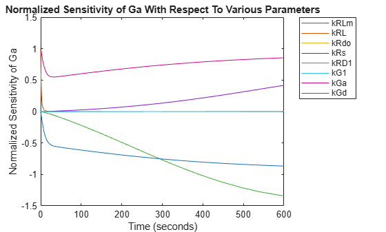
Figure contains an axes object. The axes object with title Normalized Sensitivity of Ga With Respect To Various Parameters, xlabel Time (seconds), ylabel Normalized Sensitivity of Ga contains 8 objects of type line. These objects represent kRLm, kRL, kRdo, kRs, kRD1, kG1, kGa, kGd.

From the previous plot you can see that Ga is most sensitive to parameters kGd, kRs, kRD1, and kGa. This suggests that the amounts of active G protein in the cell depends on the rate of:

Receptor synthesis
Degradation of the receptor-ligand complex
G protein activation
G protein inactivation