Scaling Virtual Calibration and System Design with parsim and AWS

This example shows you how to use Amazon Web Services (AWS) and the parsim function to scale virtual calibration and system design to run simulations in the cloud. This approach aligns with the shift to software-defined vehicle architectures, which decouple hardware and software development, enabling faster deployment of new or updated software features. This decoupling supports virtual system-level analysis, which reduces reliance on hardware-in-the-loop (HIL) and in-vehicle testing, and saves development time. Although this approach requires more computing resources and a vehicle model with detailed component-level representations, it is more efficient than traditional testing methods. By leveraging cloud resources, you can scale simulation studies, explore the entire design space, and quickly iterate to optimize design and calibration values. You can efficiently evaluate multiple design alternatives without being constrained by physical hardware.

In this example, these principles are applied in a system-level study using a configured virtual vehicle model to evaluate the feasibility of adding a Sport+ mode feature to an electric vehicle through software-only changes. Sport+ mode is intended to enhance electric vehicle performance while minimizing the impact on the miles per gallon equivalent (MPGe). The system-level study shows how to set up a large Simulink^® model and run hundreds of simulations, leveraging cloud resources and parallel computing to achieve the goals and vary the parameters specified in this table.

Study Goals	Parameters
Achieve a 0-60 mph in less than 6 seconds Quantify and minimize losses in MPGe Quantify gains from regenerative (regen) braking in different driving conditions	MaxDschrgCurrLim – Maximum allowable discharge current from the battery RegenLimits – Operational range for regen braking during braking events

The study uses a virtual two-motor electric vehicle model generated from the Virtual Vehicle Composer (Powertrain Blockset) app. The parameters are evaluated across these four drive cycles to assess their impact on energy consumption, state-of-charge (SOC) discharge rate, and maximum acceleration.

Drive Cycle	Description
Wide Open Throttle (WOT)	Simulates maximum acceleration or power demand to assess the powertrain performance under full load and fuel consumption and emissions during aggressive driving
Highway Fuel Economy Test (HWFET)	Simulates highway driving conditions for testing vehicle fuel economy and emissions
Allgemeiner Deutscher Automobil-Club Bundesautobahn (ADAC BAB)	Simulates real-world driving conditions on German autobans
Federal Test Procedure 1975 (FTP75)	Simulates urban driving conditions for testing vehicle emissions and fuel economy

To compare simulation efficiency, you can run this study using three different methods:

• Simulation in series.

• Simulation using the parsim function and Parallel Computing Toolbox™. See Running Multiple Simulations in Simulink.

• Using the parsim function with MATLAB^® Parallel Server™ on Amazon Web Services (AWS). See Run MATLAB in AWS Using Cloud Center.

This table summarizes the expected simulation time for each method.

Method	Number of Simulations	Number of Cores	Simulation Time	AWS Instance
Simulation in series	364	6	3 hours	None
Simulation using parsim and Parallel Computing Toolbox	364	6	66 minutes	MATLAB — m5.12xlarge
Simulation on MATLAB Parallel Server using parsim	364	16	12 minutes	MATLAB — m5.12xlarge MATLAB Parallel Server — m5.08xlarge with auto-resize disabled

After comparing total simulation times for each method, perform scaling studies on the cluster using the parsim function with MATLAB Parallel Server to minimize the simulation time.

Prerequisites: Set Up MATLAB Parallel Server on AWS Using Cloud Center

Prior to creating the system-level study, you must set up MATLAB on an AWS virtual machine using Cloud Center as well as MATLAB Parallel Server:

Note

An AWS account is required.

1. Link your AWS account to Cloud Center. See Link Your Cloud Account to Cloud Center.

   • Click the Follow Guided Steps option for instructions to link your cloud account.

2. Start a cloud machine with MATLAB installed. See Start MATLAB on Amazon Web Services (AWS) Using Cloud Center.

3. Create a MATLAB Parallel Server cluster in Cloud Center. See Create and Discover Clusters.

Video Walkthrough

For a walkthrough of the setup, play the video.

Video Transcript

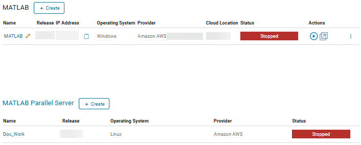
After the cloud resources are set up, the Cloud Center dashboard should look similar to this image.

Open MATLAB Cloud Instance

To open a MATLAB cloud instance, click the button located on the Cloud Center dashboard. After the cloud resources Status is set to Running, click the three dots next to the Actions button and click Open MATLAB. Then, open MATLAB from the cloud machine. The cloud can take five to 10 minutes to start.

Install Drive Cycle Data

To access the drive cycles required for this example, install the Drive Cycle Data support package from the Add-Ons explorer . The FTP75 drive cycle is available by default. To install the WOT, HWFET, and ADAC BAB drive cycles, see Install Drive Cycle Data (Powertrain Blockset).

Run System-Level Study and Analysis

This example uses a virtual vehicle model configured using Virtual Vehicle Composer (Powertrain Blockset). The vehicle model is specified to include a 340 volt battery pack (96s31p configuration) with two motors sized to meet the needs of a typical passenger vehicle. The battery management system (BMS) uses a custom-built BMS that is not available by default in Virtual Vehicle Composer.

openProject("RangeStudyUsingParameterSweep.prj");

To run the system-level study in a MATLAB® cloud instance, you must copy the project files from your local machine to the cloud machine. Then, open the project from the MATLAB cloud instance. For information on transferring files, see Transfer Data to or from MATLAB in Cloud Center.

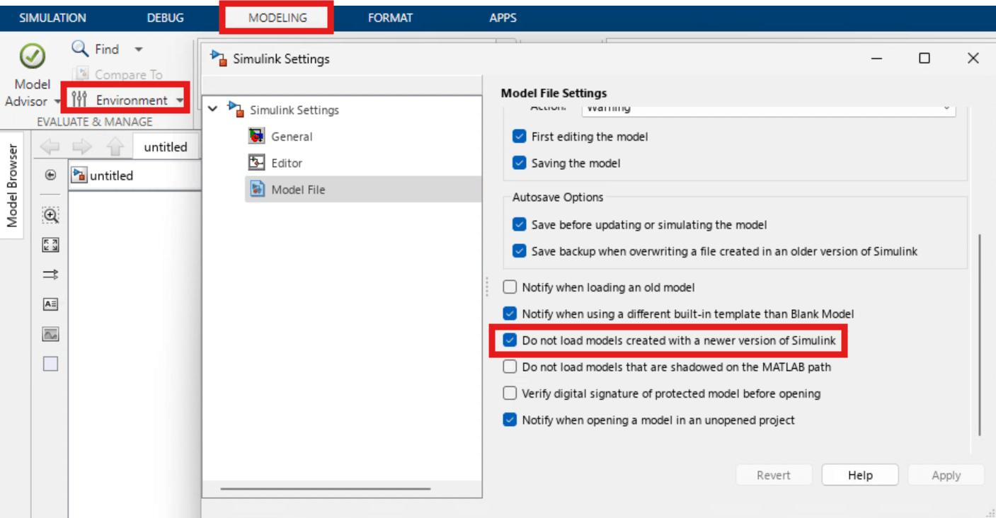
If the cloud machine does not support the latest MATLAB version, first export the data dictionary to the MATLAB version used on the cloud machine using the exportToVersion function. Then, in the MATLAB cloud instance, start Simulink®. Before loading the model, in the toolstrip, in the Evaluate & Manage section, click the down arrow next to Environment and clear the Do not load models created with a newer version of Simulink option.

Open the virtual vehicle model.

mdl = 'ConfiguredVirtualVehicleModel';
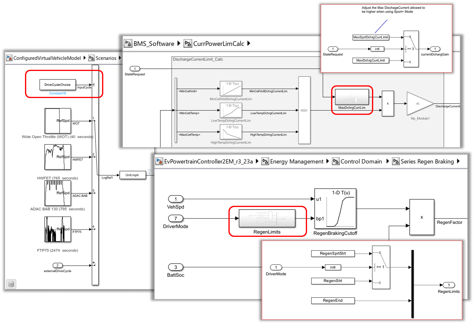
open_system(mdl);

Set Up Multi-Simulation Study

Set up a parameter sweep to test multiple combinations of parameter values to determine the optimal values for the Sport+ mode feature. Specify the range of values to be tested for the maximum discharge current limit, the operational regen range, and the drive cycle parameters.

input_MaxDchrgCurrLimit = single(-12 : -0.5: -18)';
input_RegenStrt = (2:0.5:5)';
input_DriveCycleChoice = [1 2 3 4]';
input_DriveCycleChoiceTime = [40 765 795 2474]';

Define the simulation conditions for each simulation by saving combinations of the input parameter values to a Simulink.SimulationInput object.

runID = 1;
clear in
for v1 = 1:length(input_MaxDchrgCurrLimit)
    for v2 = 1:length(input_RegenStrt)
        for v3 = 1:length(input_DriveCycleChoice)

            in(runID) = Simulink.SimulationInput(mdl);

            in(runID) = in(runID).setVariable('MaxSprtDchrgCurrLimit',input_MaxDchrgCurrLimit(v1),'Workspace','global-workspace');
            in(runID) = in(runID).setVariable('RegenSprtStrt',input_RegenStrt(v2),'Workspace','global-workspace');
            in(runID) = in(runID).setVariable('DriveCycleChoice',input_DriveCycleChoice(v3),'Workspace','global-workspace');
            in(runID) = in(runID).setModelParameter("StopTime",num2str(input_DriveCycleChoiceTime(v3)));
            
            runID = runID+1;
        end
    end
end

Run Simulations

Run a small sample of simulations in serial.

inSeries = in(1:4);
tic
set_param(mdl, 'FastRestart', 'on')
outseries = sim(inSeries, 'ShowSimulationManager', 'on');

[23-Jan-2026 14:31:18] Running simulations...
### Searching for referenced models in model 'ConfiguredVirtualVehicleModel'.
### Total of 4 models to build.
### Model reference simulation target for DriverPassThrough is up to date.
### Model reference simulation target for EvPowertrainController2EM is up to date.
### Model reference simulation target for OpenLoopBraking is up to date.
### Starting serial model build.
### Successfully updated the model reference simulation target for: BMS_Software

Build Summary

Model reference simulation targets:

Model         Build Reason                                                           Status                        Build Duration
=================================================================================================================================
BMS_Software  Global variable #MaxSprtDchrgCurrLimit#BMS_Software_DD.sldd# changed.  Code generated and compiled.  0h 0m 43.659s

1 of 4 models built (3 models already up to date)
Build duration: 0h 0m 49.732s
[23-Jan-2026 14:32:38] Completed 1 of 4 simulation runs
[23-Jan-2026 14:33:09] Completed 2 of 4 simulation runs
[23-Jan-2026 14:33:38] Completed 3 of 4 simulation runs
[23-Jan-2026 14:35:11] Completed 4 of 4 simulation runs

toc

Elapsed time is 237.337724 seconds.

Performing the same simulation studies on a quad-core laptop would take more than 5000 seconds to complete.

You can scale your simulation studies using Parallel Computing Toolbox and MATLAB Parallel Server by running simulations in parallel on different workers. Using the parsim function, you can run the same model with different inputs or different parameter settings in scenarios such as Monte Carlo analyses, parameter sweeps, model testing, experiment design, and model optimization.

To run the simulation in parallel using the parsim function, select the checkbox. To set up your environment, see Run Code on Parallel Pools (Parallel Computing Toolbox).

if true
    tic
    parpool('Processes');
    studyData = parsim(in,'ShowSimulationManager', 'on');
    delete(gcp('nocreate'))
    toc
end

[23-Jan-2026 14:49:03] Checking for availability of parallel pool...
[23-Jan-2026 14:49:03] Starting Simulink on parallel workers...
[23-Jan-2026 14:50:29] Loading project on parallel workers...
[23-Jan-2026 14:50:29] Configuring simulation cache folder on parallel workers...
[23-Jan-2026 14:50:50] Loading model on parallel workers...
[23-Jan-2026 14:53:52] Running simulations...
[23-Jan-2026 15:39:51] Cleaning up parallel workers...

Parallel pool using the 'Processes' profile is shutting down.

Elapsed time is 3947.458847 seconds.

To run the simulations at scale on the cluster created in Cloud Center using the parsim function and MATLAB Parallel Server, select the checkbox. To set up your environment, see Scale Up from Desktop to Cluster (Parallel Computing Toolbox). Replace Doc_Work with the name of your parallel server profile.

if false
    tic 
    parpool('Doc_Work'); 
    studyData = parsim(in(1:364),'ShowSimulationManager', 'on'); 
    delete(gcp('nocreate'));
    toc
end

Review Simulation Time

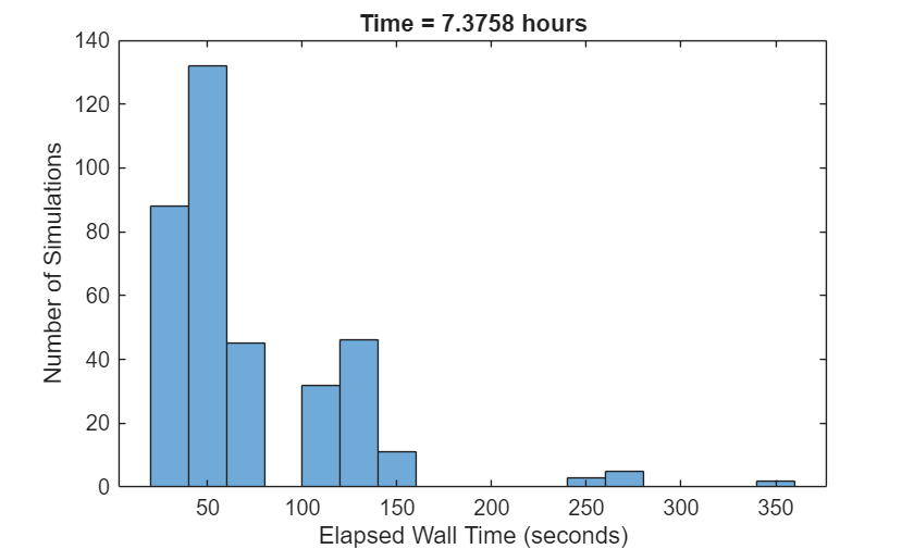
Generate a histogram showing the distribution of simulation run times. Include a title that displays the total cumulative time spent across all simulations.

figure
totaltime = zeros(1,length(studyData));
for i = 1:length(studyData)
    totaltime(i) = studyData(i).SimulationMetadata.TimingInfo.TotalElapsedWallTime;
end
histogram(totaltime);
xlabel('Elapsed Wall Time (seconds)');
ylabel('Number of Simulations');title(['Time = ' num2str(sum(totaltime)/3600) ' hours']);

clear i totaltime;

Review Simulation Results

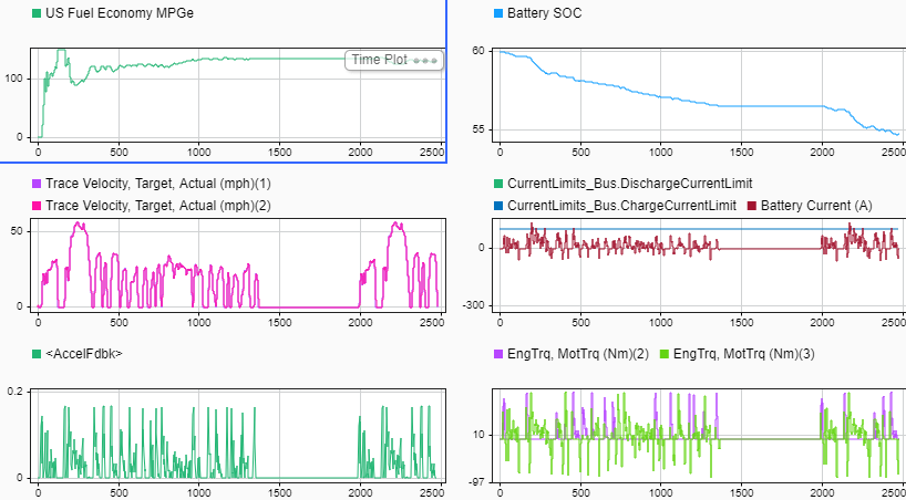
Plot the simulation results for one of the simulation objects using the Simulation Data Inspector template provided, VirtualVehicleData.mldatx.

plot(studyData(1,4))
Simulink.sdi.loadView(fullfile('Scripts','SystemSimStudy','VirtualVehicleData.mldatx'))

Reduce 0-60 mph Time

Use the slider to inspect the simulation results to observe the effect different regen lower limit values have on meeting the target velocity for each drive cycle.

sigName = 'Trace Velocity, Target, Actual (mph)';
regenTbl_Low =5;
plotCommonRegenTbl(sigName,regenTbl_Low,studyData, input_MaxDchrgCurrLimit,input_RegenStrt);

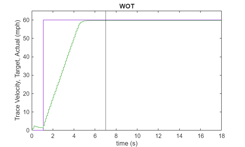
When you inspect the WOT test using the acceleration plot, you can observe the effect the maximum allowable discharge current value has on the vehicle from 0 to 60 mph. As the current discharge value increases, you see a gain in acceleration time. The curves begin to deviate at higher speeds because, at low speeds, you are not limited by current or power, but by how much torque you are allowed to apply to limit wheel speed at launch.

plotAccelerationUpdate(studyData, input_MaxDchrgCurrLimit,input_RegenStrt)

Minimize Losses in MPGe

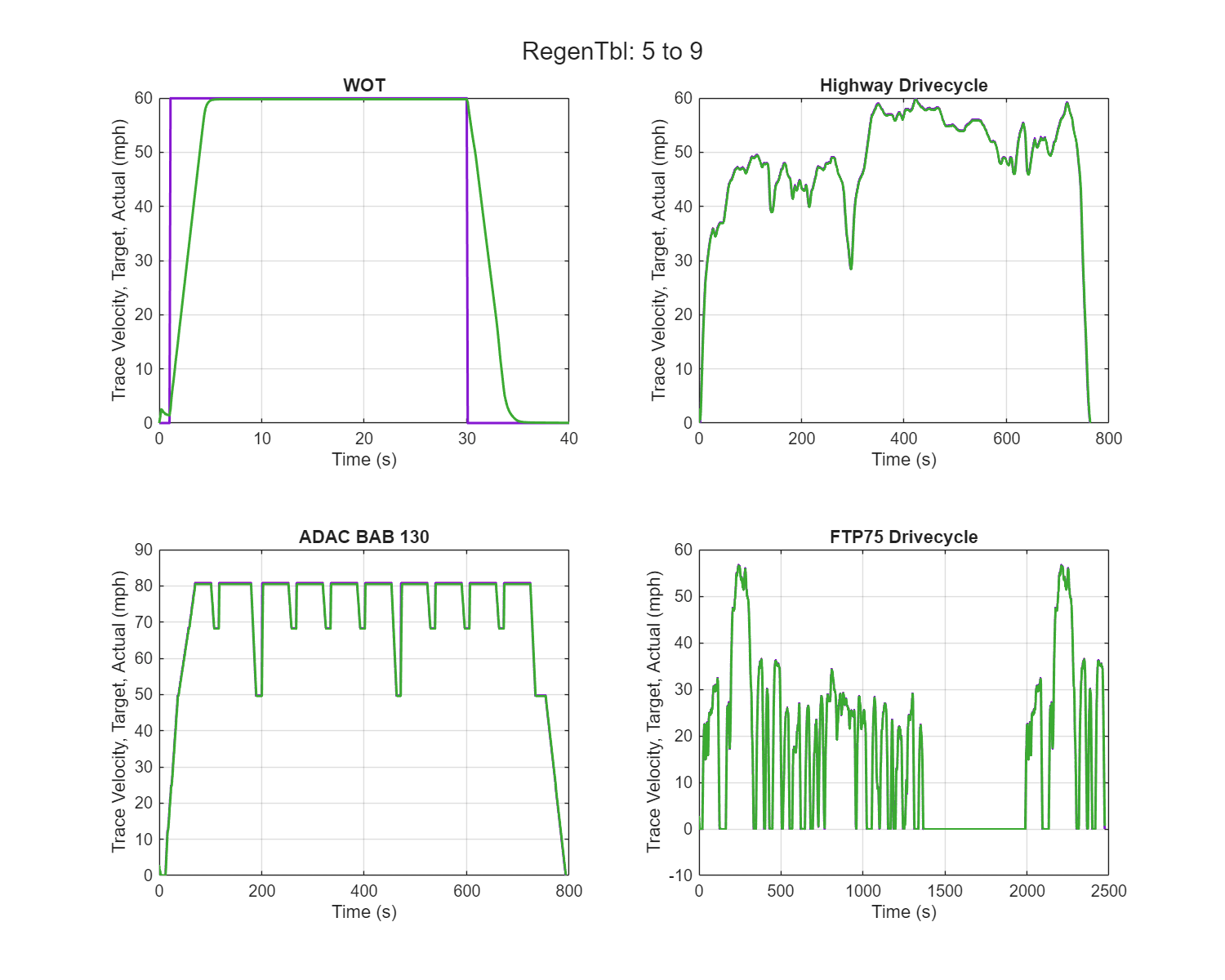
Use the slider to inspect the simulation results to observe the effect different regen lower limit values have on MPGe.

sigName = 'US Fuel Economy MPGe';
regenTbl_Low =5;
plotCommonRegenTbl(sigName,regenTbl_Low,studyData, input_MaxDchrgCurrLimit,input_RegenStrt);

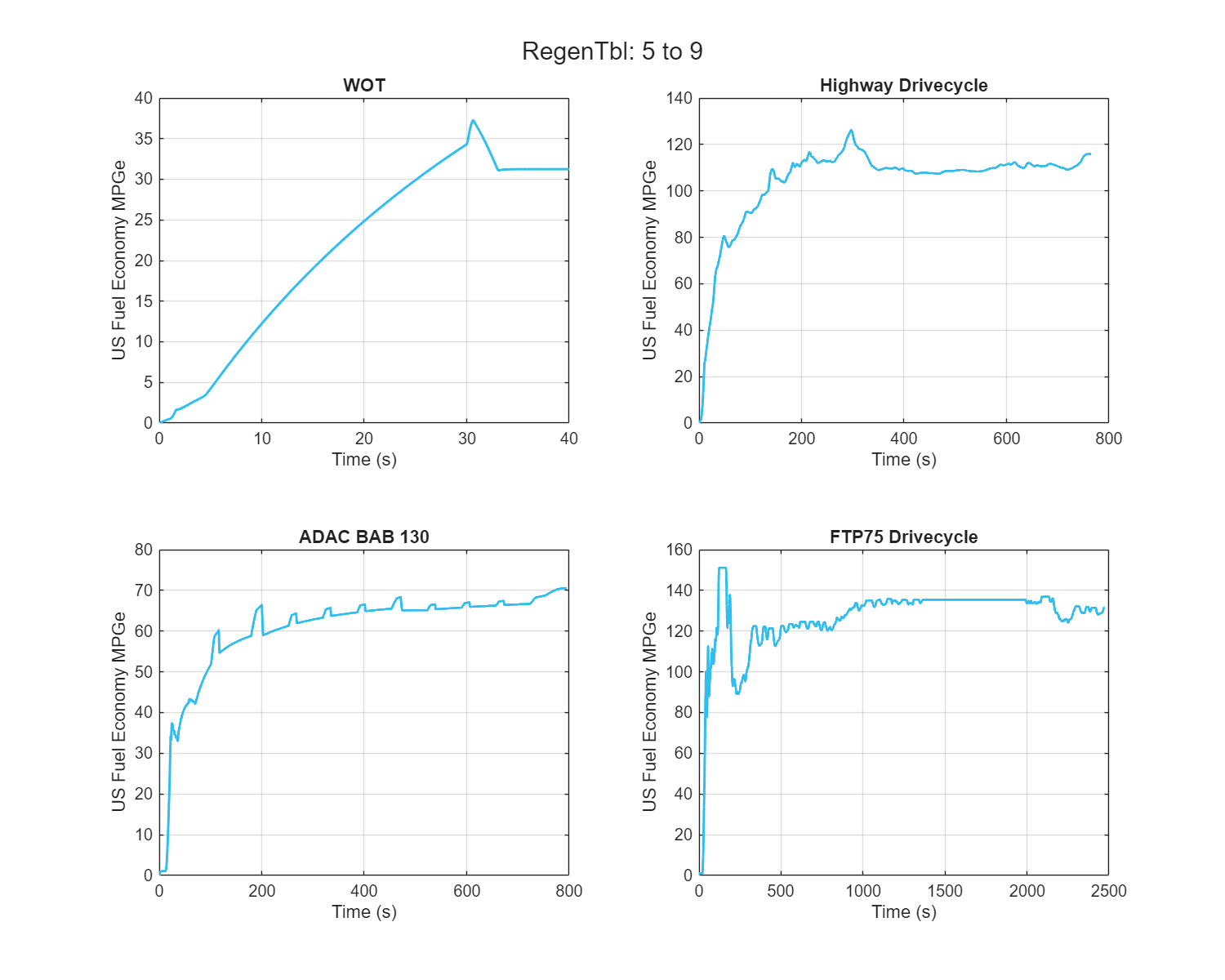
Increasing the current results in higher energy consumption, which reduces the EV range on the WOT and ADAC drive cycles.

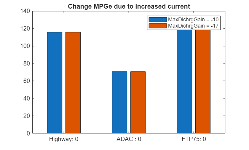
Over 15-minute drive cycles in Sport+ mode, a 0.5% increase adds up quickly. You can offset this gain by recovering more energy during braking.

sigName         = 'US Fuel Economy MPGe';
baserun         = 25;  % Run Corresponding to RegenTblLow = 5; gainMaxDschrgCur = -10
highCurRun      = 221; % Run Corresponding to RegenTblLow = 5; gainMaxDschrgCur = -17
plotValChange(sigName,baserun,highCurRun,studyData)

Increase EV Range

Changing the regenTbl_Low value extends the range in which the regen is operational.

figure
hold on
fill([5 9 9], [0 1 0], [0.9 0.9 0.5], 'FaceAlpha', 0.5, 'EdgeColor', 'none', 'HandleVisibility','off');
fill([2.5 9 9], [0 1 0], [0.5 0.7 0.9], 'FaceAlpha', 0.5, 'EdgeColor', 'none', 'HandleVisibility','off');
plot([5,9],[0,1],'b','LineWidth',2)
plot([2.5,9],[0,1],'r','LineWidth',2)
title('Regen Operating Region')
legend('Baseline','Modified','Location','northwest')
hold off

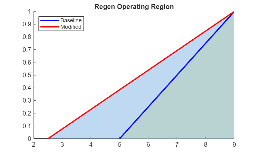
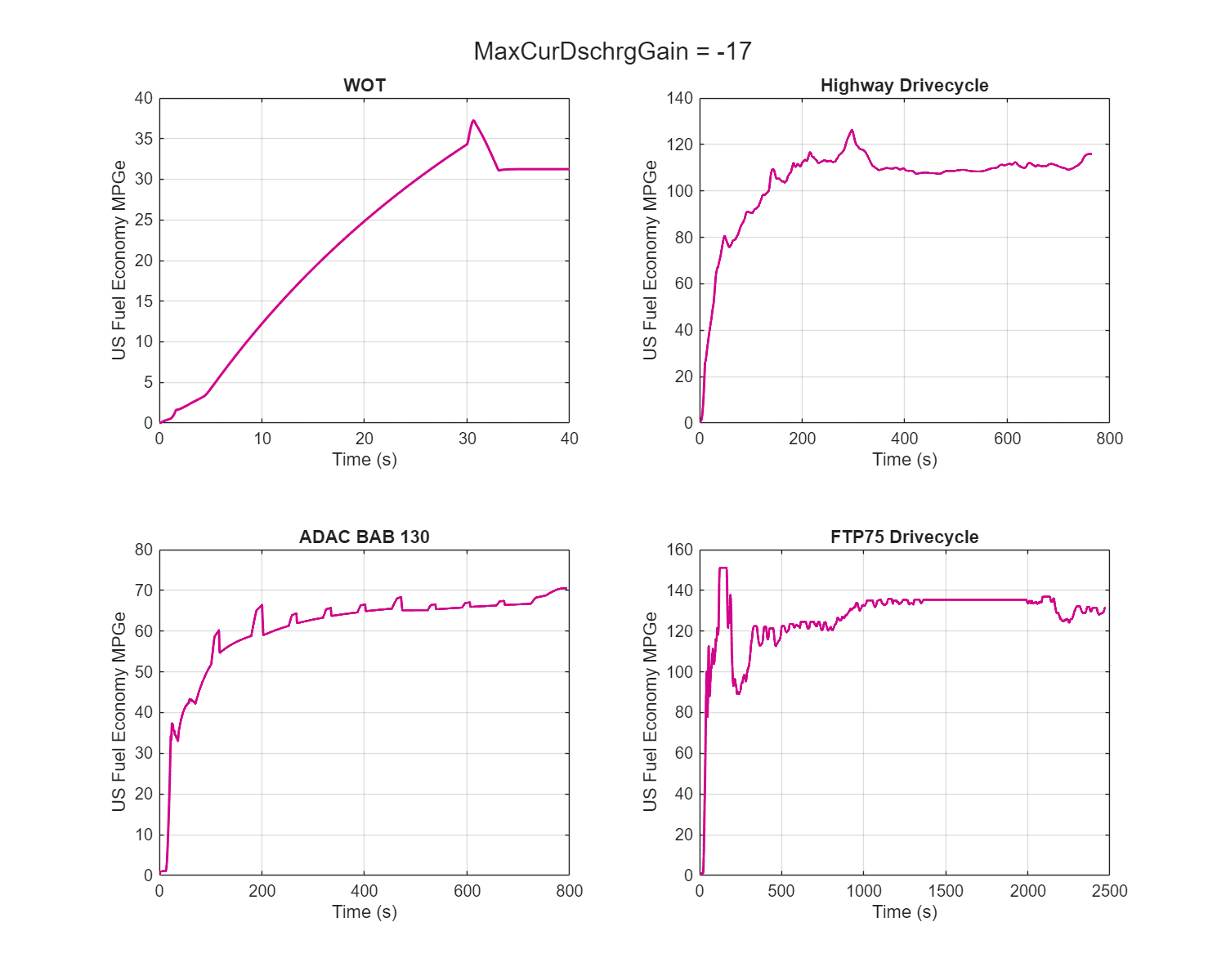
Varying the regen range shows no MPGe gains in highway or low-braking cycles, but gives improvements during hard braking, as seen in WOT, city, or traffic driving.

sigName = 'US Fuel Economy MPGe';
maxDischargeGain =-17;
plotCommonDischrg(sigName,maxDischargeGain, studyData, input_MaxDchrgCurrLimit,input_RegenStrt);

To view the simulation plot functions used in the analysis, in SystemSimulationStudy/Scripts, go to the HelperFunctions folder.

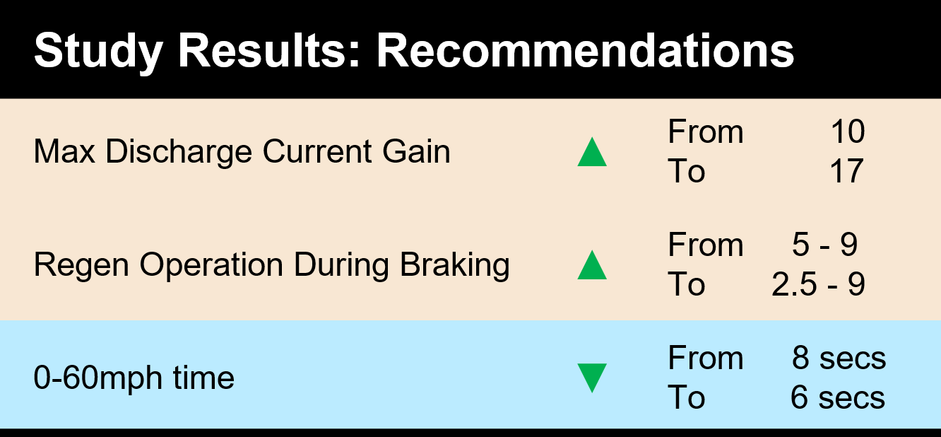
Inferences from the Study Data

Increasing the allowed discharge current by 70% enables a 0–60 mph time under 6 seconds. To offset the higher energy use during acceleration and maintain MPGe, you can reduce the regen lower limit from 5 to 2.5 to expand regenerative braking.