Design a Guidance System in MATLAB and Simulink
This example shows how to use the model of the missile airframe presented in a number of published papers on the use of advanced control methods applied to missile autopilot design. See [1], [2], and [3]. The model represents a tail-controlled missile traveling between Mach 2 and Mach 4, at altitudes ranging between 10,000 ft (3,050 m) and 60,000 ft (18,290 m), with typical angles of attack ranging between +/- 20 degrees.
Airframe Dynamics Model
The core element of the model is a nonlinear representation of the rigid body dynamics of the airframe. The aerodynamic forces and moments acting on the missile body are generated from coefficients that are non-linear functions of both incidence and Mach number.
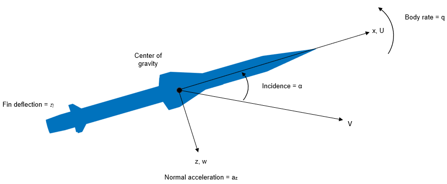
Create the model using Simulink® and the Aerospace Blockset™. The Aerospace Blockset provides reference components, such as atmosphere models, that are common to all models irrespective of the airframe configuration.
Open the model.

Represent Airframe in Simulink
The airframe model consists of four principal subsystems, controlled through the acceleration-demand autopilot. The Atmosphere & Incidence, Airspeed Computation subsystem calculates the change in atmospheric conditions with changing altitude. The Fin Actuator and Sensors subsystems couple the autopilot to the airframe. The Aerodynamics & Equations of Motion subsystem calculates the magnitude of the forces and moments acting on the missile body and integrates the equations of motion.

International Standard Atmosphere Model
The Atmosphere & Incidence Airspeed Computation subsystem approximates the International Standard Atmosphere (ISA) and is split into two regions. The troposphere region lies between sea level and 11 km and has a linear temperature drop that corresponds to changing altitude. The lower stratosphere region ranges between 11 km and 20 km and has a constant temperature.

Aerodynamic Coefficients for Forces and Moments
The Aerodynamics & Equations of Motion subsystem generates the forces and moments applied to the missile in body axes and integrates the equations of motion that define the linear and angular motion of the airframe.

The aerodynamic coefficients are stored in datasets. During the simulation, the value at the current operating condition is determined by interpolation using 2-D Lookup Table blocks.

Classical Three-Loop Autopilot Design
The missile autopilot controls acceleration normal to the missile body. In this example, the autopilot structure is a three-loop design that uses measurements from an accelerometer placed ahead of the center of gravity. A rate gyro provides additional damping. The controller gains are scheduled on incidence and Mach number and are tuned for robust performance at an altitude of 10,000 ft.
Designing the autopilot using classical design techniques requires that linear models of the airframe pitch dynamics be derived about a number of trimmed flight conditions. MATLAB® can determine the trim conditions, and derive linear state space models directly from the nonlinear Simulink model. This method saves time and helps to validate the model. The functions provided by the MATLAB Control System Toolbox™ and Simulink® Control Design™ allow you to visualize the behavior of the airframe open-loop frequency (or time) responses. To see how to trim and linearize the airframe model, see Airframe Trim and Linearize (Simulink).
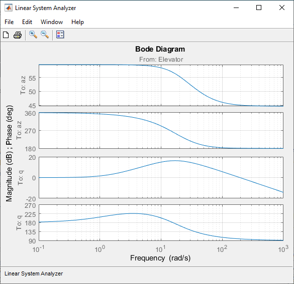
Airframe Frequency Response
Autopilot designs are carried out on a number of linear airframe models derived at varying flight conditions across the expected flight envelope. To implement the autopilot in the nonlinear model, you must store the autopilot gains in two-dimensional lookup tables and incorporate an anti-windup gain to prevent integrator windup when the fin demands exceed the maximum limits. You can then test the autopilot in the nonlinear Simulink model to show satisfactory performance in the presence of nonlinearities such as actuator fin and rate limits and with the gains dynamically varying with changing flight conditions. The Autopilot subsystem implements the gain schedule.
Homing Guidance Loop
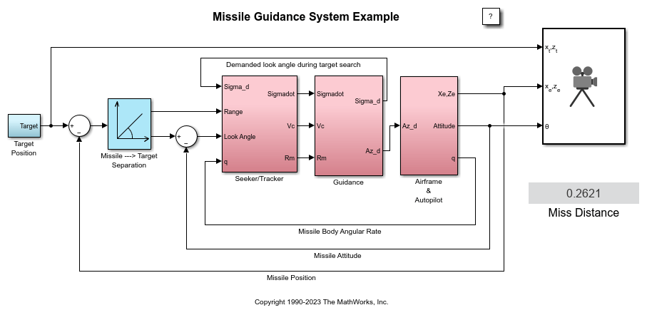
The homing guidance loop contains a Seeker/Tracker subsystem that returns measurements of the relative motion between the missile and target. The Guidance subsystem generates normal acceleration demands which are passed to the autopilot. The autopilot becomes part of an inner loop within the overall homing guidance system. For information on the differing forms of guidance and background information on the analysis techniques that are used to quantify guidance loop performance, see [4].

Guidance Subsystem
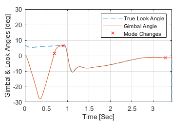
The Guidance subsystem generates demands during closed-loop tracking and perform an initial search to locate the target position. A Stateflow® chart controls the transfer between these differing modes of operation. Switching between modes is triggered by events generated either in Simulink or internal to the Stateflow chart. You can control the behavior of the Simulink model by changing the value of Mode. This variable is used to switch between differing control demands. During target search, the Stateflow chart controls the tracker directly by sending demands to the seeker gimbals (Sigma). The tracker flags target acquisition once the target lies within the beamwidth of the seeker (Acquire). After a short delay, closed-loop guidance starts. Stateflow functionality enables the system to rapidly define all operational modes, for example, actions to take should when a loss of lock on the target occurs or when a target is not acquired during target search.

Proportional Navigation Guidance
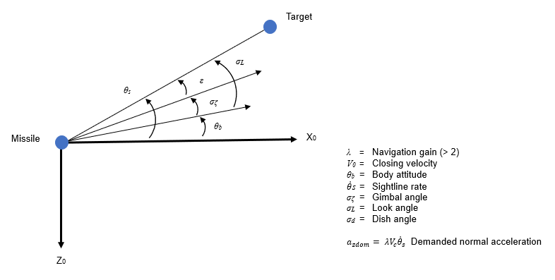
Once the seeker has acquired the target, a proportional navigation guidance (PNG) law is used to guide the missile until impact. This form of guidance law has been used in guided missiles since the 1950s and can be applied to radar, infrared, or television guided missiles. The navigation law requires these data:
Measurements of the closing velocity between the missile and target, which can be obtained using a Doppler tracking device for a radar-guided missile
An estimate for the rate of change of the inertial sightline angle
Seeker/Tracker Subsystem
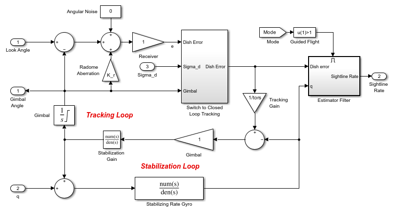
The Seeker/Tracker subsystem drives the seeker gimbals to keep the seeker dish aligned with the target and provides the guidance law with an estimate of the sightline rate. The tracker loop time constant tors is set to 0.05 s and represents a compromise between maximizing speed of response and keeping noise transmission within acceptable levels. The stabilization loop compensates for body rotation rates. The gain Ks, which is the loop crossover frequency, is set as high as possible subject to the limitations of the bandwidth of the stabilizing rate gyro. The sightline rate estimate is a filtered value of the sum of the rate of change of the dish angle measured by the stabilizing rate gyro and an estimated value for the rate of change of the angular tracking error (e) measured by the receiver. In this example, the bandwidth of the estimator filter is set to half the bandwidth of the autopilot.
Radome Aberration
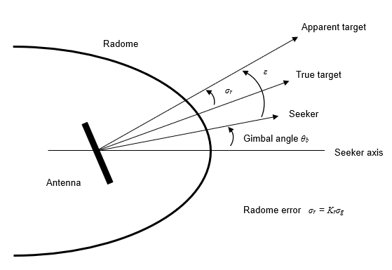
For radar-guided missiles, a commonly modeled parasitic feedback effect is radome aberration. Radome aberration occurs when the shape of the protective covering over the seeker distorts the returning signal and gives a false reading of the look angle to the target. Generally, the amount of distortion is a nonlinear function of the current gimbal angle. However, the model approximates a linear relationship between the gimbal angle and the magnitude of the distortion using a Gain block named Radome Aberration. You can also model other parasitic effects, such as sensitivity in the rate gyros to normal acceleration, to test the robustness of the target tracker and estimator filters.
Run Guidance Simulation
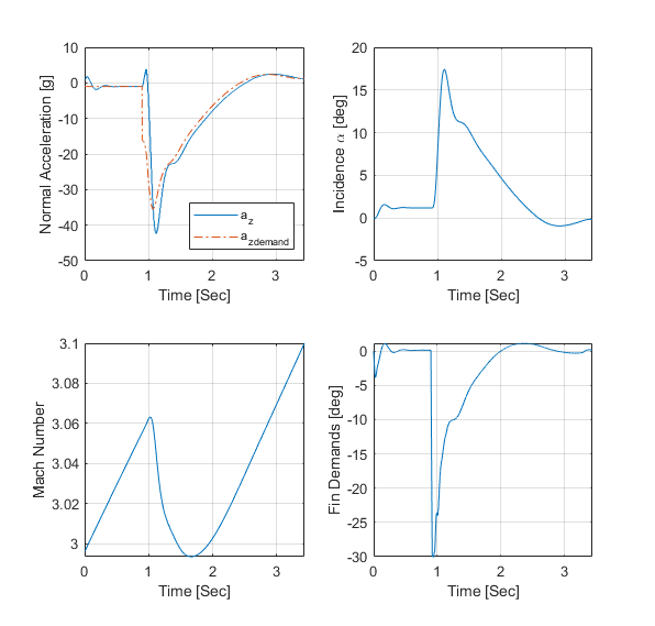
You can now test the performance of the overall system. The target is defined to be traveling at a constant speed of 328 m/s on a course reciprocal to the initial missile heading and 500 m above the initial missile position. Simulation results show that acquisition occurs at 0.69 seconds into the engagement, with closed-loop guidance starting after 0.89 seconds. Impact with the target occurs at 3.46 seconds, and the range to go at the point of closest approach is 0.265 m.
The aero_guid_plot.m script runs a performance analysis.

The animation block provides a visual reference for the simulation.

