2-D Wavelet Compression
R2026bThis section takes you through the features of wavelet 2-D true compression using the Wavelet Toolbox™ software.
For more information on the compression methods see Wavelet Compression for Images in the Wavelet Toolbox User's Guide.
For more information on the main function available when using command-line mode, see
the wcompress reference pages.
Starting from a given image, the goal of the true compression is to minimize the length of the sequence of bits needed to represent it, while preserving information of acceptable quality. Wavelets contribute to effective solutions for this problem.
The complete chain of compression includes phases of quantization, coding and decoding in addition of the wavelet processing itself.
Perform Image Compression
The purpose of this section is to show how to compress and uncompress a grayscale or truecolor image using various compression methods.
In this section, you will learn to
Compress using global thresholding and Huffman encoding
Uncompress
Compress using progressive methods
Handle truecolor images
Compression by Global Thresholding and Huffman Encoding
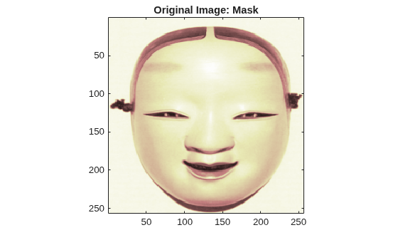
First load and display the grayscale image mask.
load mask
image(X)
axis square
colormap(pink(255))
title("Original Image: Mask")
A synthetic performance of the compression is given by the compression ratio and the Bit-Per-Pixel ratio which are equivalent.
The compression ratio CR means that the compressed image is stored using only CR% of the initial storage size.
The Bit-Per-Pixel ratio BPP gives the number of bits used to store one pixel of the image.
For a grayscale image, the initial BPP is 8 while for a truecolor image the initial BPP is 24 because 8 bits are used to encode each of the three colors (RGB color space).
The challenge of compression methods is to find the best compromise between a weak compression ratio and a good perceptual result.
Let us begin with a simple method cascading global coefficients thresholding and Huffman encoding. We use the default wavelet bior4.4 and the default level which is the maximum possible level (see the wmaxlev function) divided by 2.
Set the desired Bit-Per-Pixel ratio BPP to 0.5. Store the compressed image in the file mask.wtc.
meth = "gbl_mmc_h";   % Method name
option = "c";         % "c" stands for compression
[CR,BPP] = wcompress(option,X,"mask.wtc",meth,bpp=0.5)
CR =
6.7200
BPP =
0.5376
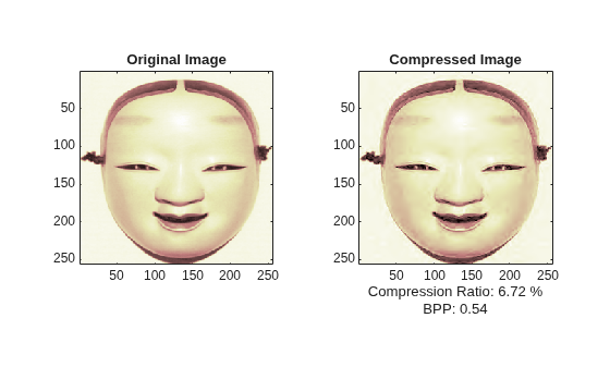
The achieved Bit-Per-Pixel ratio is actually about 0.53 (closed to the desired one) for a compression ratio of 6.7%.
Uncompress Image
Uncompress the image retrieved from the file mask.wtc and compare it to the original image.
option = "u";       % "u" stands for uncompression
Xc = wcompress(option,'mask.wtc');
figure
tiledlayout(1,2)
colormap(pink(255))
nexttile
image(X)
axis square
title("Original Image")
nexttile
image(Xc)
axis square
title("Compressed Image")
xlabel({"Compression Ratio: "+num2str(CR,'%1.2f %%'), ...
    "BPP: "+num2str(BPP,'%3.2f')})
Compression by Progressive Methods
Let us now illustrate the use of progressive methods starting with the well known EZW algorithm using the Haar wavelet. The key parameter is the number of loops. Increasing it leads to better recovery but worse compression ratio.
meth = "ezw";     % Method name
Wname  = "haar";  % Wavelet name
nbloop = 6;       % Number of loops
[CR,BPP] = wcompress("c",X,"mask.wtc",meth, ...
    maxloop=nbloop,wname=Wname);
Xc = wcompress("u","mask.wtc");
figure
tiledlayout(1,2)
colormap(pink(255))
nexttile
image(X)
axis square
title("Original Image")
nexttile
image(Xc)
axis square
title("Compressed Image - 6 Steps")
xlabel({"Compression Ratio: "+num2str(CR,'%1.2f %%'), ...
    "BPP: "+num2str(BPP,'%3.2f')})
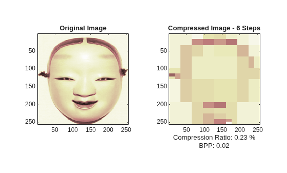
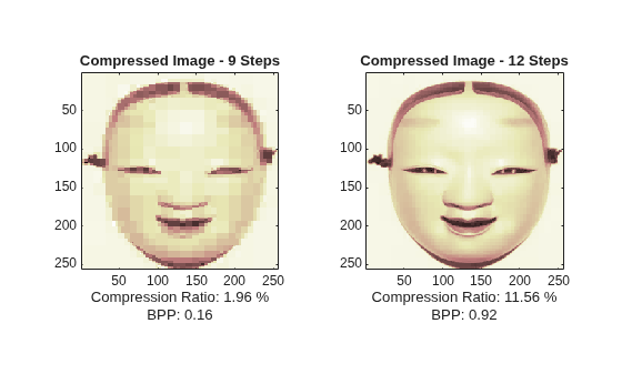
A too small number of steps (here 6) produces a very coarse compressed image. So let us examine a little better result for 9 steps and a satisfactory result for 12 steps. As can be seen, the reached BPP ratio is about 0.92 when using 12 steps.
[CR,BPP]= wcompress("c",X,"mask.wtc",meth,maxloop=9, ...
    wname="haar");
Xc = wcompress("u","mask.wtc");
figure
tiledlayout(1,2)
colormap(pink(255))
nexttile
image(Xc)
axis square
title("Compressed Image - 9 Steps")
xlabel({"Compression Ratio: "+num2str(CR,'%1.2f %%'), ...
    "BPP: "+num2str(BPP,'%3.2f')})

[CR,BPP] = wcompress("c",X,"mask.wtc",meth,maxloop=12, ...
    wname="haar");
Xc = wcompress("u","mask.wtc");
nexttile
image(Xc)
axis square
title("Compressed Image - 12 Steps")
xlabel({"Compression Ratio: "+num2str(CR,'%1.2f %%'), ...
    "BPP: "+num2str(BPP,'%3.2f')})
Let us try to improve the previous result by using the wavelet bior4.4 instead of haar and looking at obtained results for steps 12 and 11.
[CR,BPP]= wcompress("c",X,"mask.wtc","ezw",maxloop=12, ...
    wname="bior4.4");
Xc = wcompress("u","mask.wtc");
figure
tiledlayout(1,2)
colormap(pink(255))
nexttile
image(Xc)
axis square
title("Compressed Image - 12 Steps - bior4.4")
xlabel({"Compression Ratio: "+num2str(CR,'%1.2f %%'), ...
    "BPP: "+num2str(BPP,'%3.2f')})

[CR,BPP] = wcompress("c",X,"mask.wtc","ezw",maxloop=11, ...
    wname="bior4.4");
Xc = wcompress("u","mask.wtc");
nexttile
image(Xc)
axis square
title("Compressed Image - 11 Steps - bior4.4")
xlabel({"Compression Ratio: "+num2str(CR,'%1.2f %%'), ...
    "BPP: "+num2str(BPP,'%3.2f')})
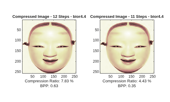
Starting from the eleventh loop, the result can be considered satisfactory. The reached BPP ratio is now about 0.35. It can even be slightly improved by using a more recent method: SPIHT (Set Partitioning In Hierarchical Trees).
[CR,BPP] = wcompress("c",X,"mask.wtc","spiht",maxloop=12, ...
    wname="bior4.4");
Xc = wcompress("u","mask.wtc");
figure
tiledlayout(1,2)
colormap(pink(255))
nexttile
image(X)
axis square
title("Original Image")
nexttile
image(Xc)
axis square
title("Compressed Image - 12 Steps - bior4.4")
xlabel({"Compression Ratio: "+num2str(CR,'%1.2f %%'), ...
    "BPP: "+num2str(BPP,'%3.2f')})
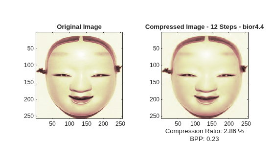
Use measerr to obtain the quality metrics of the image approximation.
[psnr,mse,maxerr,l2rat] = measerr(X,Xc)
psnr =
32.8601
mse =
33.6564
maxerr =
59.3447
l2rat =
0.9949
Delete the compressed image.
delete("mask.wtc")The final compression ratio (2.8%) and the Bit-Per-Pixel ratio (0.23) are very satisfactory. Let us recall that the first ratio means that the compressed image is stored using only 2.8% of the initial storage size.
Handling Truecolor Images
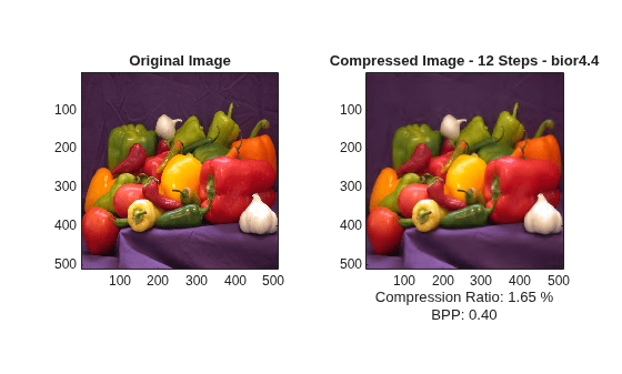
Finally, let us illustrate how to compress the wpeppers.jpg truecolor image. Truecolor images can be compressed along the same scheme as the grayscale images by applying the same strategies to each of the three color components.
X = imread("wpeppers.jpg");
[CR,BPP] = wcompress("c",X,"wpeppers.wtc","spiht",maxloop=12);
Xc = wcompress("u","wpeppers.wtc");
figure
tiledlayout(1,2)
nexttile
image(X)
axis square
title("Original Image")
nexttile
image(Xc)
axis square
title("Compressed Image - 12 Steps - bior4.4")
xlabel({"Compression Ratio: "+num2str(CR,'%1.2f %%'), ...
    "BPP: "+num2str(BPP,'%3.2f')})
Delete the compressed image.
delete("wpeppers.wtc")The compression ratio (1.65%) and the Bit-Per-Pixel ratio (0.4) are very satisfactory while maintaining a good visual perception.

