Design And Analyze Spherically Capped Biconical Antenna

This example shows how to model and analyze a spherically capped biconical antenna using custom 3-D shapes. This antenna is a canonical broadband radiator used in practical ultra-wide-band communication systems. [1] The two cones of the antenna are connected by a cylindrical delta gap feed. The height and diameter of the cylindrical feed are equal. The location of the feed is chosen in between the two cone apex points as the gap between them can be considered as infinitesimally small, which nearly resembles an ideal antenna. Later, the effect of feed dimensions variation and mesh density variation near the delta gap is studied by comparing the antenna input impedance for two different feed diameters and mesh density. The antenna is analyzed in the frequency range of 900MHz to 15GHz.

Define Cone, Sphere, and Feed Dimensions

Define the sphere radius, cone radius and height, feed height, width, and diameter in meters. Define the frequency range in Hertz for antenna analysis.

sphereRadius = 0.024;
coneCapRadius = 0.017;
coneHeight = 0.017;
feedHeight1 = 0.5e-3;
feedHeight2 = 0.08e-3;
feedWidth1 = 0.5e-3;
feedWidth2 = 0.02e-3;
feedDia1 = feedWidth1; 
feedDia2 = feedWidth2;
freq = linspace(0.9e9,15e9,30);

Create Bicone Geometry

Create the cone, spherical caps and the feed geometry and add them to generate the spherically capped bicone.

Create Cone

Create the cone with shape.Cylinder shape using the defined dimensions with different radii (one for spherical cap and one for feed) on each cap. Keep both the caps open to attach them to the other shapes. Move the shape near to the feed location.

cone1 = shape.Cylinder(Cap=[0 0],Height=coneHeight,...
    Radius=[feedDia1/2 coneCapRadius]);
translate(cone1,[0 0 coneHeight/2+feedHeight1/2]);

Create Feed Geometry

Use the defined dimensions to create the feed geometry.

feed1 = shape.Cylinder(Cap=[0 0],Height=feedHeight1/2,...
    Radius=feedDia1/2);
feed1 = translate(feed1,[0 0 feedHeight1/4]);

Connect Feed to Cone

Use Boolean add operation to connect the feed to the cone.

ConeNfeed1 = add(feed1,cone1);

Add Spherical Caps

Create a sphere of radius of 0.024m. Perform intersect operation on this sphere and the cone created in the above steps to form spherically capped cone structure.

sph1 = shape.Sphere(Radius=sphereRadius);
capShape1 = intersect(ConeNfeed1,sph1);

Add Bottom Cone to Spherically Capped Cone

Copy the spherically capped cone and rotate it to align with the feed. Perform add operation on these two spherical capped cones to join them and form a biconical structure.

capShape1Copy = copy(capShape1);
[~] = rotate(capShape1Copy,180,[0 0 0],[0 1 0]);
antShape1 = add(capShape1,capShape1Copy,RetainShape=false);
show(antShape1);

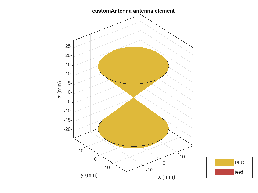
Create Spherically Capped Bicone Antenna

Convert the biconical structure into an antenna by using customAntenna and add feed point to it using createFeed function.

ant1 = customAntenna(Shape=antShape1);
[~] = createFeed(ant1,[0 0 0],20);
show(ant1)

Analyze Biconical Antenna

Manually mesh the biconical antenna and analyze the impedance behavior over the 900MHz-15GHz frequency range. Also analyze the current distribution of the antenna.

[~] = mesh(ant1,MaxEdgeLength=0.0012);
i1 = impedance(ant1,freq);
figure
current(ant1,7.7e9,Scale="log10");

Compare Impedance Behavior for Different Feed Diameters

Create a similar biconical antenna with 0.02mm feed diameter.

cone2 = shape.Cylinder(Cap=[0 0],Height=coneHeight,...
    Radius=[feedDia2/2 coneCapRadius]);
translate(cone2,[0 0 coneHeight/2+feedHeight2/2]);

Create feed geometry.

feed2 = shape.Cylinder(Cap=[0 0],Height=feedHeight2/2,...
    Radius=feedDia2/2);
feed2 = translate(feed2,[0 0 feedHeight2/4]);

Connect feed to cone.

ConeNfeed2 = add(feed2,cone2);

Add spherical caps.

sph2 = shape.Sphere(Radius=sphereRadius);
capShape2 = intersect(ConeNfeed2,sph2);

Add bottom cone to spherical capped cone.

capShape2Copy = copy(capShape2);
[~] = rotate(capShape2Copy,180,[0 0 0],[0 1 0]);
antShape2 = add(capShape2,capShape2Copy,RetainShape=false);
show(antShape2);

Convert the biconical structure into an antenna by using customAntenna and add feed point to it using createFeed function.

ant2 = customAntenna(Shape=antShape2);
[~] = createFeed(ant2,[0 0 0],20);
show(ant2)

Manually mesh the biconical antenna and analyze the impedance behavior over the 900MHz-15GHz frequency range. Compare and plot the impedance behavior of this antenna with the antenna having 0.5mm feed diameter.

[~] = mesh(ant2,MaxEdgeLength=0.001,MinEdgeLength=1e-5);
i2 = impedance(ant2,freq);

Compare impedance results for 0.5mm and 0.02mm feed diameters.

plot(freq,real(i1),Color="b");
hold on;
plot(freq,real(i2),'--',Color="b");
hold on;
plot(freq,imag(i1),Color="r");
hold on;
plot(freq,imag(i2),'--',Color="r");
grid on
legend("Resistance (dia = 0.5mm)","Resistance (dia = 0.02mm)","Reactance (dia = 0.5mm)","Reactance (dia = 0.02mm)",Location="southeast");
xlabel("Frequency (Hz)");
ylabel("Impedance (ohms)");
hold off

Conclusion

A broadband biconical antenna is constructed using custom 3-D shapes and it is observed that, the feed dimensions variation and mesh density variation near the delta gap causes significant variations in the antenna input impedance. This analysis helps you to fine tune the feed dimensions and mesh density for your application.

References

[1] Zheng, Shucheng, Peiyuan Zhang, and Vladimir I. Okhmatovski. “Analysis of Benchmark Biconical Antenna with RWG Method of Moments for IEEE P2816 Project.” In 2022 IEEE International Symposium on Antennas and Propagation and USNC-URSI Radio Science Meeting (AP-S/URSI), 649–50. Denver, CO, USA: IEEE, 2022. https://doi.org/10.1109/AP-S/USNC-URSI47032.2022.9886141.