Current Visualization on Antenna Surface

Create Dipole Antenna

Design the dipole antenna to resonate around 1 GHz. The wavelength at this frequency is 30 cm. The dipole length is equal to half-wavelength, which corresponds to 15 cm. The width of the dipole strip is chosen to be 5 mm.

mydipole = dipole(Length=15e-2, Width=5e-3);
show(mydipole);

Calculate Current Distribution on Dipole Surface

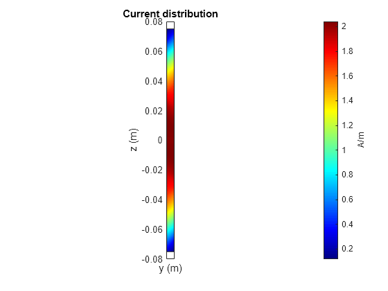
Since the dipole length is 15 cm, choose the operation frequency as $$f=c/(2*l)$$, where c is the speed of light. A current distribution in the form of the half period of a sine wave along the dipole length is observed with the maximum occurring at the antenna center. A periodic current distribution along the dipole is further observed with multiple maxima and minima at higher resonant frequencies (2f, 3f,...). This periodic current distribution is typical for dipoles and similar resonant wire antennas [1].

c = 2.99792458e8;
f = c/(2*mydipole.Length);
current(mydipole, f);
view(90,0);

Calculate and Plot Individual Current Components

Specify the output arguments in the function current and access the individual current components. The vector points correspond to the triangle centers where the current values are evaluated. The plot below displays the longitudinal (z) component and the transverse (y) component of the surface current density magnitude.

[C, points]  = current(mydipole, f);
Jy = abs(C(2,:));
Jz = abs(C(3,:));
figure;
plot(points(3,:), Jz, 'r*', points(3,:), Jy, 'b*');
grid on;
xlabel('Dipole length (m)')
ylabel('Surface current density, A/m');
legend('|Jz|', '|Jy|');

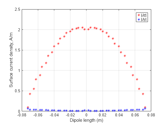
This current distribution is typical in the MoM analysis [1], [2]. Better (smoother) results will be obtained with finer triangular surface meshes and when the current is plotted exactly on the centerline of the strip.

Place the Dipole in Front of Reflector

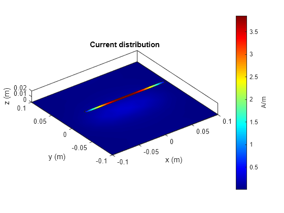
Place the dipole in front of a finite planar reflector by choosing the dipole antenna as an exciter for the reflector antenna. Orient the dipole so that it is parallel to the reflector. This is done by modifying the tilt of the exciter (the dipole) so that it now lies along the x-axis. A tilt of 90 degrees is applied about the Y axis to achieve this. The spacing between the dipole and reflector is chosen to be 2 cm.

myreflector = reflector(Exciter=mydipole, Spacing=0.02);
myreflector.Exciter.Tilt = 90;
myreflector.Exciter.TiltAxis = [0 1 0];
current(myreflector, f);

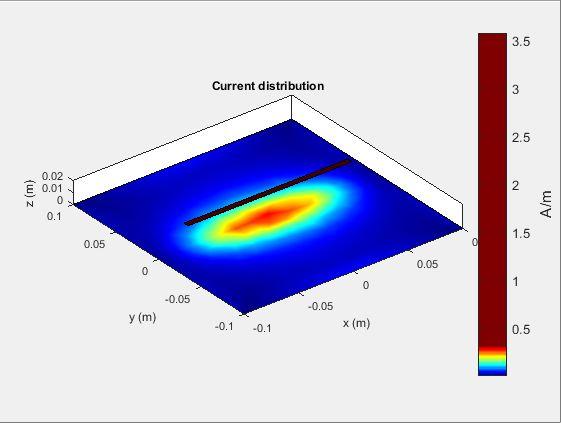
Currents are also induced on the reflector surface as shown in the figure above. To better visualize the currents on the reflector surface, hover the mouse on the color bar and change the dynamic range (scale) of the current plot as explained below.

Interaction with Color Bar

Hover the mouse over the color bar. The mouse arrow is now transformed into a flat arrow. Pull the mouse up or down to change the dynamic range of the current. This helps us to better visualize the current distribution on the reflector surface as shown below. You can also pull the magnitude of the currents next to the color bar to change the dynamic range.

Right click on the color bar and select the Reset limit tab to change the current limits to the original values. There is also an option to change the colormap and move the color bar to a different location as shown below.

References

[1] C. A. Balanis, 'Antenna Theory. Analysis and Design,' Wiley, New York, 3rd Edition, 2005.

[2] S. N. Makarov, 'Antenna and EM Modeling with MATLAB,' p.66, Wiley & Sons, 2002.