Reconstruct 3-D Radiation Pattern of 5G Phased Array from Sparse Measurements Using AI

R2026b

Since R2026b

This example demonstrates how to reconstruct the full 3-D radiation pattern of a 5G mmWave phased array antenna from a small number of measurement cuts. The reconstruction employs the artificial intelligence (AI) based patternFromAI function from Antenna Toolbox™ to infer full 3-D patterns from sparse observations. The workflow simulates a practical over-the-air (OTA) testing scenario with the following constraints and considerations:

• Only a few 2-D pattern slices are available from chamber measurements

• The full 3-D pattern must be inferred from this sparse data

• Pattern multiplication enables array-level characterization from element-level measurements

The example uses synthetic data generated from full-wave simulation of a 28 GHz patch antenna array to provide a ground-truth reference for evaluating reconstruction accuracy. In practice, the sparse slice data would come from physical measurements in an anechoic chamber.

Background

OTA characterization of 5G mmWave phased arrays in anechoic chambers is time-consuming and expensive. A full 3-D pattern measurement at 1-degree resolution requires over 65,000 sample points. By contrast, capturing two elevation cuts and one azimuthal cut at 2-degree resolution yields approximately 540 samples — a 120x reduction in measurement time.

The patternFromAI function uses a pretrained deep learning model to reconstruct a plausible 3-D pattern from such sparse observations. The model has been trained on a diverse corpus of antenna and array patterns from the Antenna Toolbox catalog and has learned the general structure of physical radiation patterns on the sphere.

This example evaluates reconstruction accuracy for the following scenarios:

1. A single patch element (simpler pattern structure)

2. A uniform array (narrower beams, sidelobe structure)

3. An array pattern estimated via pattern multiplication from the reconstructed element

4. A beamsteered array (asymmetric main beam, off-broadside peak)

Overview of Measurement Data

The example uses three data sets generated from full-wave simulation of a 28 GHz patch element, a 4x4 rectangular array with uniform excitation, and a beamsteered variant of the same array. Each data set contains the full 3-D directivity pattern on a 1-degree grid (360 azimuth by 181 elevation points) and sparse measurement slices sampled at 2-degree resolution. The baseline configuration consists of two elevation cuts at azimuth 0 degrees and 90 degrees, respectively, and one azimuthal cut at elevation 0 degrees (i.e. the horizon). The steered case includes an additional targeted elevation cut through the steering direction. Note that each elevation cut traces a full 360-degree path through both poles by extending the elevation angle beyond the conventional $$\pm$$90-degree range. These sparse slices represent the limited data acquired in a practical OTA chamber measurement, where full 3-D pattern sweeps can be prohibitively time-consuming. Refer to the companion script generate28GHzPatchArrayPatternData.m for details.

Load and Visualize Element Measurement Data

Load the measurement data for a 28 GHz microstrip patch element.

elemData = load("patchElement_28GHz_patternData.mat");
disp(elemData.description)

28 GHz patchMicrostrip, 0.7*lambda ground plane

Visualize the element measurement slices.

figure
polarpattern(elemData.elcut1.el,elemData.elcut1.data,TitleTop="Element — Elevation Cut (az = 0 deg)")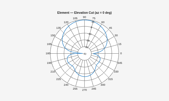

figure
polarpattern(elemData.elcut2.el,elemData.elcut2.data,TitleTop="Element — Elevation Cut (az = 90 deg)")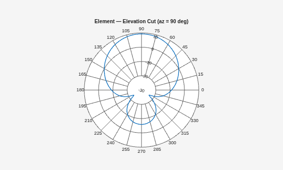

figure
polarpattern(elemData.azcut.az,elemData.azcut.data,TitleTop="Element — Azimuthal Cut (el = 0 deg)")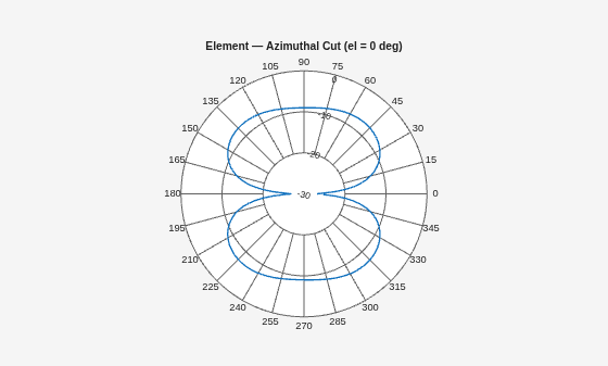

Reconstruct Element 3-D Pattern from Sparse Measurements

Assemble the sparse measurement samples into the vectors required by patternFromAI: directivity values in dBi, azimuth angles, and elevation angles. Each sample is a triplet (magnitude, azimuth, elevation). The extended elevation convention (beyond $$\pm$$90 degrees) is accepted directly.

elemSparseData = [elemData.elcut1.data,elemData.elcut2.data,elemData.azcut.data];
elemSparseAz = [elemData.elcut1.az*ones(size(elemData.elcut1.el)), ...
    elemData.elcut2.az*ones(size(elemData.elcut2.el)),elemData.azcut.az];
elemSparseEl = [elemData.elcut1.el,elemData.elcut2.el,zeros(size(elemData.azcut.az))];
nSparse = numel(elemSparseData);
nFull = 360*181;
disp("Sparse samples: " + nSparse + " (from " + nFull + "-point grid)")

Sparse samples: 542 (from 65160-point grid)

disp("Compression: " + round(nFull/nSparse) + "x")

Compression: 120x

Reconstruct the full 3-D pattern from the sparse samples.

[elemRecon,elOut,azOut] = patternFromAI(elemSparseData, ...
    elemSparseAz,elemSparseEl,AngleConvention="az-el");

Visualize Reconstructed and Reference Element Patterns

Import the reconstructed pattern into a measuredAntenna object using the helperMeasuredAntennaFromDirectivity local function. This readily facilitates both 3-D visualization here and pattern multiplication later.

azVec = double(azOut);
elVec = double(elOut);
[azGrid,elGrid] = meshgrid(azVec,elVec);
azGrid = azGrid.';
elGrid = elGrid.';
dirMat = [azGrid(:),elGrid(:),ones(numel(azGrid),1)];
mElemRecon = helperMeasuredAntennaFromDirectivity(elemRecon(:),dirMat,elemData.freq,azVec,elVec);

Visualize the reconstructed pattern. Set the magnitude scale to a 40 dB dynamic range below the reference peak to subsequently enable direct visual comparison with the reference pattern.

elemPeakRef = max(elemData.p3D(:));
pOptsElem = PatternPlotOptions(MagnitudeScale=[elemPeakRef-40,elemPeakRef]);
figure
pattern(mElemRecon,elemData.freq,azVec,elVec,PatternOptions=pOptsElem)
title("Element Pattern — AI Reconstruction")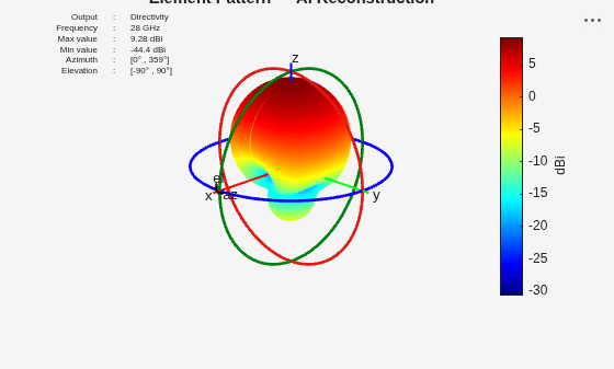

Compare against the reference pattern.

mElemRef = helperMeasuredAntennaFromDirectivity(elemData.p3D(:),dirMat,elemData.freq,azVec,elVec);
figure
pattern(mElemRef,elemData.freq,azVec,elVec,PatternOptions=pOptsElem)
title("Element Pattern — Reference")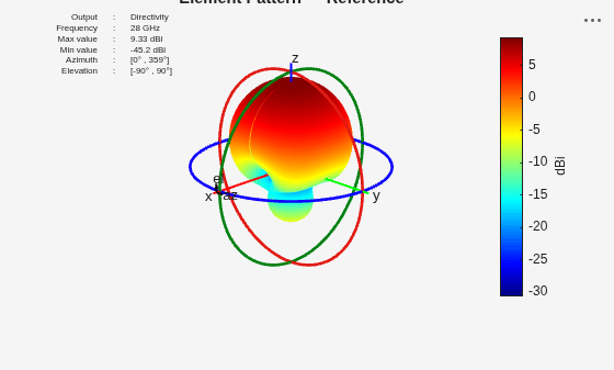

Evaluate Element Reconstruction Accuracy

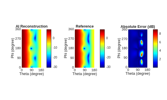
Calculate the root-mean-squared error (RMSE) and mean absolute error (MAE) over the full 3-D pattern to quantify overall reconstruction accuracy.

elemAbsErr = abs(elemRecon - elemData.p3D);
elemRMSE = sqrt(mean(elemAbsErr.^2,"all"));
elemMAE = mean(elemAbsErr,"all");
disp("Element RMSE: " + round(elemRMSE,2) + " dB")

Element RMSE: 1.14 dB

disp("Element MAE:  " + round(elemMAE,2) + " dB")

Element MAE:  0.56 dB

Visualize the spatial error distribution.

figure
tiledlayout(1,3)
nexttile
helperPatternCustomRectangular(elemRecon,90-elVec,azVec, ...
    Title="AI Reconstruction",MagnitudeScale=[elemPeakRef-40 elemPeakRef])
nexttile
helperPatternCustomRectangular(elemData.p3D,90-elVec,azVec, ...
    Title="Reference",MagnitudeScale=[elemPeakRef-40 elemPeakRef])
nexttile
helperPatternCustomRectangular(elemAbsErr,90-elVec,azVec, ...
    Title="Absolute Error (dB)")

Load and Visualize Array Measurement Data

Load the measurement data for a 4x4 uniform rectangular array at 28 GHz with 0.7$$\lambda$$ element spacing. The array pattern has narrower beams and more sidelobe structure than the element.

arrData = load("patchArray4x4_28GHz_uniformPatternData.mat");
disp(arrData.description)

4x4 rectangular array, 0.7*lambda spacing, uniform excitation

Visualize the array measurement slices.

figure
polarpattern(arrData.elcut1.el,arrData.elcut1.data,TitleTop="Array — Elevation Cut (az = 0 deg)")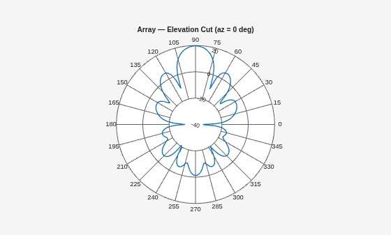

figure
polarpattern(arrData.elcut2.el,arrData.elcut2.data,TitleTop="Array — Elevation Cut (az = 90 deg)")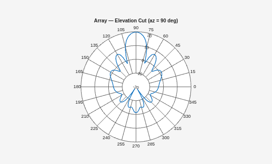

figure
polarpattern(arrData.azcut.az,arrData.azcut.data,TitleTop="Array — Azimuthal Cut (el = 0 deg)")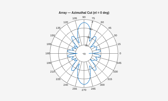

Reconstruct Array 3-D Pattern from Sparse Measurements

Assemble the sparse measurements and reconstruct the array pattern.

arrSparseData = [arrData.elcut1.data,arrData.elcut2.data,arrData.azcut.data];
arrSparseAz = [arrData.elcut1.az*ones(size(arrData.elcut1.el)), ...
    arrData.elcut2.az*ones(size(arrData.elcut2.el)),arrData.azcut.az];
arrSparseEl = [arrData.elcut1.el,arrData.elcut2.el,zeros(size(arrData.azcut.az))];
[arrRecon,~,~] = patternFromAI(arrSparseData, ...
    arrSparseAz,arrSparseEl,AngleConvention="az-el");

Visualize Reconstructed and Reference Array Patterns

Import the reconstructed pattern into a measuredAntenna object.

mArrRecon = helperMeasuredAntennaFromDirectivity(arrRecon(:),dirMat,arrData.freq,azVec,elVec);

Visualize the reconstructed array pattern. Set the magnitude scale to a 40 dB dynamic range below the reference peak, which captures the main beam, sidelobes, and the upper portion of the null structure while suppressing noise-floor clutter.

arrPeakRef = max(arrData.p3D(:));
pOpts = PatternPlotOptions(MagnitudeScale=[arrPeakRef-40,arrPeakRef]);
figure
pattern(mArrRecon,arrData.freq,azVec,elVec,PatternOptions=pOpts)
title("Array Pattern — AI Reconstruction")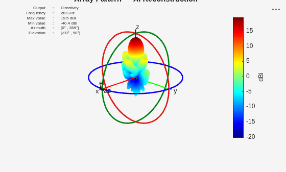

Compare against the reference pattern.

mArrRef = helperMeasuredAntennaFromDirectivity(arrData.p3D(:),dirMat,arrData.freq,azVec,elVec);
figure
pattern(mArrRef,arrData.freq,azVec,elVec,PatternOptions=pOpts)
title("Array Pattern — Reference")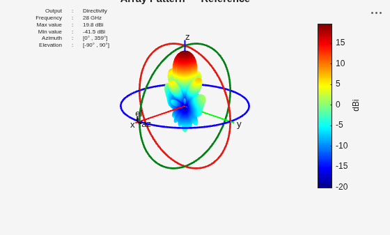

Evaluate Array Reconstruction Accuracy

Compute the reconstruction error.

arrAbsErr = abs(arrRecon - arrData.p3D);
arrRMSE = sqrt(mean(arrAbsErr.^2,"all"));
arrMAE = mean(arrAbsErr,"all");
disp("Array RMSE: " + round(arrRMSE,2) + " dB")

Array RMSE: 5.13 dB

disp("Array MAE:  " + round(arrMAE,2) + " dB")

Array MAE:  3.14 dB

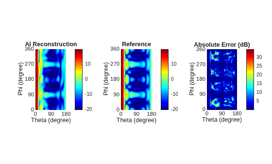
Visualize the spatial error distribution.

figure
tiledlayout(1,3)
nexttile
helperPatternCustomRectangular(arrRecon,90-elVec,azVec, ...
    Title="AI Reconstruction",MagnitudeScale=[arrPeakRef-40 arrPeakRef])
nexttile
helperPatternCustomRectangular(arrData.p3D,90-elVec,azVec, ...
    Title="Reference",MagnitudeScale=[arrPeakRef-40 arrPeakRef])
nexttile
helperPatternCustomRectangular(arrAbsErr,90-elVec,azVec, ...
    Title="Absolute Error (dB)")

Compare Element and Array Reconstruction Error Distribution

Compare element and array reconstruction accuracy on the same axes using the cumulative distribution of absolute error. This directly shows the fraction of angular coordinates that fall below a given error threshold.

elemErrSorted = sort(elemAbsErr(:));
arrErrSorted = sort(arrAbsErr(:));
nPts = numel(elemErrSorted);
cdfPct = (1:nPts).'/nPts*100;
figure
hElem = stairs(elemErrSorted,cdfPct,DisplayName="Element");
hold on
hArr = stairs(arrErrSorted,cdfPct,DisplayName="Array (uniform)");
hold off
idx3dB_elem = find(elemErrSorted<=3,1,"last");
idx3dB_arr = find(arrErrSorted<=3,1,"last");
datatip(hElem,DataIndex=idx3dB_elem,Location="southeast");
datatip(hArr,DataIndex=idx3dB_arr,Location="southeast");
xlabel("Absolute Error (dB)")
ylabel("Percentage of Angular Coordinates")
title("Cumulative Distribution of Reconstruction Error")
legend(Location="southeast")
grid on

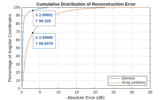
The datatips mark the 3 dB error threshold: 96% of angular coordinates have less than 3 dB error for the element, and 69% for the array. The element pattern, with its broad smooth structure, is substantially easier to reconstruct than the array pattern, whose narrow beams and deep nulls are more challenging for the model to recover from sparse observations.

Estimate Array Pattern Using Pattern Multiplication

Pattern multiplication decomposes the array pattern into the product of the element pattern and the array factor. If the element pattern can be reconstructed from sparse measurements, the full array pattern can be obtained by applying the known array geometry — without measuring the array at all.

The reconstructed element measuredAntenna created earlier includes an E-field derived from directivity assuming linear polarization and zero phase. These assumptions are reasonable for a linearly polarized patch element and enable patternMultiply to compute the array factor coherently.

Construct a rectangularArray using the reconstructed element and the known array geometry, then call patternMultiply to estimate the array pattern.

arrFromRecon = rectangularArray(Element=mElemRecon,Size=[4 4], ...
    RowSpacing=arrData.spacing,ColumnSpacing=arrData.spacing);
[arrPM,~,~] = patternMultiply(arrFromRecon,arrData.freq,azVec,elVec);

Visualize the pattern multiplication result.

arrPM = arrPM.';
mArrPM = helperMeasuredAntennaFromDirectivity(arrPM(:),dirMat,arrData.freq,azVec,elVec);
figure
pattern(mArrPM,arrData.freq,azVec,elVec,PatternOptions=pOpts)
title("Array Pattern — Pattern Multiplication")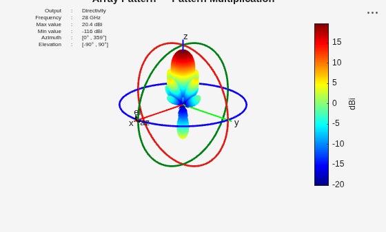

Compute the estimation error and compare to the AI reconstruction. Pattern multiplication applies exact superposition, so it predicts beam shape and peak directivity accurately. Its errors concentrate in deep null regions and in the back hemisphere, where mutual coupling, finite-array truncation effects, and ground plane diffraction cause the embedded element pattern to deviate from the isolated-element assumption.

arrPMErr = abs(arrPM - arrData.p3D);
arrPMRMSE = sqrt(mean(arrPMErr.^2,"all"));
arrPMMAE = mean(arrPMErr,"all");
disp("Pattern multiplication RMSE (full sphere): " + round(arrPMRMSE,2) + " dB")

Pattern multiplication RMSE (full sphere): 12.39 dB

disp("Pattern multiplication MAE (full sphere):  " + round(arrPMMAE,2) + " dB")

Pattern multiplication MAE (full sphere):  8.18 dB

Evaluate the accuracy within the main beam and sidelobe region, defined as within 10 dB of the peak, where pattern multiplication excels.

mainBeamMask = arrData.p3D >= (arrPeakRef - 10);
disp("Within 10 dB of peak:")

Within 10 dB of peak:

disp("  AI reconstruction MAE:       " + round(mean(arrAbsErr(mainBeamMask)),2) + " dB")

  AI reconstruction MAE:       0.93 dB

disp("  Pattern multiplication MAE:  " + round(mean(arrPMErr(mainBeamMask)),2) + " dB")

  Pattern multiplication MAE:  0.36 dB

The two approaches have complementary strengths. Pattern multiplication excels in the main beam region because it applies physics-based superposition exactly, while direct AI reconstruction captures mutual coupling effects that pattern multiplication ignores, yielding lower overall RMSE.

Reconstruct Beamsteered Array Pattern Directly from Sparse Measurements

In 5G NR beam management, the array is steered to different directions using phase tapering. Load the measurement data for the array steered to azimuth 30 degrees, elevation 60 degrees.

arrSteeredData = load("patchArray4x4_28GHz_steeredPatternData.mat");
disp(arrSteeredData.description)

4x4 rectangular array, 0.7*lambda spacing, steered to [az=30, el=60]

Attempt reconstruction using the two standard elevation cuts plus one azimuthal cut. Note that none of these cuts pass through the steered beam peak.

steeredSparseData = [arrSteeredData.elcut1.data,arrSteeredData.elcut2.data,arrSteeredData.azcut.data];
steeredSparseAz = [arrSteeredData.elcut1.az*ones(size(arrSteeredData.elcut1.el)), ...
    arrSteeredData.elcut2.az*ones(size(arrSteeredData.elcut2.el)),arrSteeredData.azcut.az];
steeredSparseEl = [arrSteeredData.elcut1.el,arrSteeredData.elcut2.el,zeros(size(arrSteeredData.azcut.az))];
[steeredRecon,~,~] = patternFromAI(steeredSparseData, ...
    steeredSparseAz,steeredSparseEl,AngleConvention="az-el");

Visualize the reconstruction from standard cuts.

steeredPeak = max(arrSteeredData.p3D(:));
pOptsSteered = PatternPlotOptions(MagnitudeScale=[steeredPeak-40,steeredPeak]);
mSteered = helperMeasuredAntennaFromDirectivity(steeredRecon(:),dirMat,arrData.freq,azVec,elVec);
figure
pattern(mSteered,arrData.freq,azVec,elVec,PatternOptions=pOptsSteered)
title("Steered Array — AI, Two Elevation Cuts")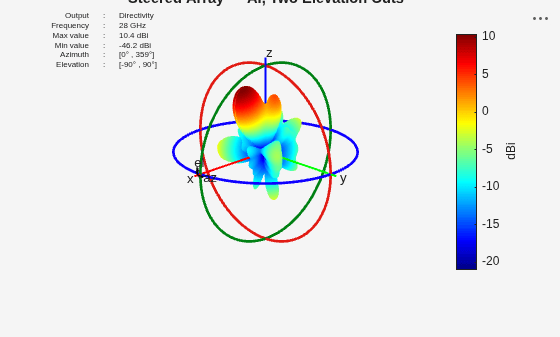

Compare against the reference pattern.

mSteeredRef = helperMeasuredAntennaFromDirectivity(arrSteeredData.p3D(:),dirMat,arrData.freq,azVec,elVec);
figure
pattern(mSteeredRef,arrData.freq,azVec,elVec,PatternOptions=pOptsSteered)
title("Steered Array — Reference")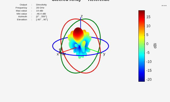

Compute the reconstruction error.

steeredAbsErr = abs(steeredRecon - arrSteeredData.p3D);
steeredRMSE = sqrt(mean(steeredAbsErr.^2,"all"));
disp("Steered (two elevation cuts + one azimuthal cut):")

Steered (two elevation cuts + one azimuthal cut):

disp("  RMSE: " + round(steeredRMSE,2) + " dB")

  RMSE: 6.6 dB

disp("  Reconstructed peak: " + round(max(steeredRecon(:)),1) + " dBi")

  Reconstructed peak: 10.4 dBi

disp("  Actual peak: " + round(max(arrSteeredData.p3D(:)),1) + " dBi")

  Actual peak: 19 dBi

The reconstruction clearly underestimates the main beam. The standard cuts do not pass through the steered beam peak, so the maximum observed directivity in the sparse data is much lower than the actual peak. The model cannot recover amplitude information absent from the input.

Improve Reconstruction with Additional Targeted Measurement Cut

Add a third elevation cut at azimuth 30 degrees, which passes directly through the steered beam. When the beam is steered off-broadside, standard principal-plane cuts may miss the main lobe entirely, so this targeted cut provides the model with amplitude information near the peak. It also demonstrates the flexibility of patternFromAI — measurements need not be restricted to principal planes.

steeredSparseDataExtraCut = [steeredSparseData,arrSteeredData.elcut3.data];
steeredSparseAzExtraCut = [steeredSparseAz,arrSteeredData.elcut3.az*ones(size(arrSteeredData.elcut3.el))];
steeredSparseElExtraCut = [steeredSparseEl,arrSteeredData.elcut3.el];
disp("Samples: two elevation + one azimuthal = " + numel(steeredSparseData) + ...
    ", three elevation + one azimuthal = " + numel(steeredSparseDataExtraCut))

Samples: two elevation + one azimuthal = 542, three elevation + one azimuthal = 723

[steeredReconExtraCut,~,~] = patternFromAI(steeredSparseDataExtraCut, ...
    steeredSparseAzExtraCut,steeredSparseElExtraCut,AngleConvention="az-el");

Visualize the improved reconstruction.

mSteeredExtraCut = helperMeasuredAntennaFromDirectivity(steeredReconExtraCut(:),dirMat,arrData.freq,azVec,elVec);
figure
pattern(mSteeredExtraCut,arrData.freq,azVec,elVec,PatternOptions=pOptsSteered)
title("Steered Array — AI, Three Elevation Cuts")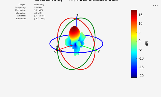

Evaluate the improvement in reconstruction accuracy.

steeredAbsErrExtraCut = abs(steeredReconExtraCut - arrSteeredData.p3D);
steeredRMSEExtraCut = sqrt(mean(steeredAbsErrExtraCut.^2,"all"));
disp("Steered (three elevation cuts + one azimuthal cut):")

Steered (three elevation cuts + one azimuthal cut):

disp("  RMSE: " + round(steeredRMSEExtraCut,2) + " dB")

  RMSE: 5.21 dB

disp("  Reconstructed peak: " + round(max(steeredReconExtraCut(:)),1) + " dBi")

  Reconstructed peak: 18.1 dBi

disp("  Actual peak: " + round(max(arrSteeredData.p3D(:)),1) + " dBi")

  Actual peak: 19 dBi

Estimate Beamsteered Array Pattern Using Pattern Multiplication

As an alternative approach, use the reconstructed element pattern with pattern multiplication. This offers a measurement-free path to steered beam characterization — apply the known steering phase shifts to the reconstructed element to obtain the full steered pattern without any steered-array measurements.

Construct the steered array as before for the uniform array, but now specify PhaseShift to apply the beam steering.

arrSteeredFromRecon = rectangularArray(Element=mElemRecon,Size=[4 4], ...
    RowSpacing=arrData.spacing,ColumnSpacing=arrData.spacing, ...
    PhaseShift=arrSteeredData.phaseShift);
[steeredPM,~,~] = patternMultiply(arrSteeredFromRecon,arrData.freq,azVec,elVec);

Visualize the steered pattern multiplication result.

steeredPM = steeredPM.';
mSteeredPM = helperMeasuredAntennaFromDirectivity(steeredPM(:),dirMat,arrData.freq,azVec,elVec);
figure
pattern(mSteeredPM,arrData.freq,azVec,elVec,PatternOptions=pOptsSteered)
title("Steered Array — Pattern Multiplication")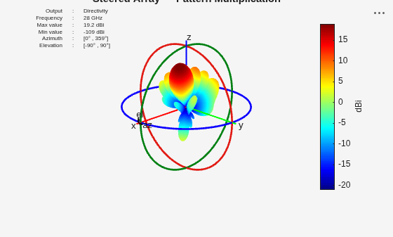

Compute the estimation error.

steeredPMErr = abs(steeredPM - arrSteeredData.p3D);
steeredPMRMSE = sqrt(mean(steeredPMErr.^2,"all"));
disp("Steered pattern multiplication RMSE: " + round(steeredPMRMSE,2) + " dB")

Steered pattern multiplication RMSE: 13.21 dB

disp("Steered pattern multiplication peak: " + round(max(steeredPM(:)),1) + " dBi" + ...
    " (actual: " + round(max(arrSteeredData.p3D(:)),1) + " dBi)")

Steered pattern multiplication peak: 19.2 dBi (actual: 19 dBi)

Pattern multiplication correctly predicts the steered beam peak and direction because it applies the known phase shifts analytically. It achieves this without any steered-array measurements — only the element pattern and array geometry are needed.

Summary

Tabulate the reconstruction accuracy across all scenarios.

scenarios = ["Element (two elevation + one azimuthal)"; ...
             "Array, uniform (two elevation + one azimuthal)"; ...
             "Array, pattern multiplication"; ...
             "Array, steered (two elevation + one azimuthal)"; ...
             "Array, steered (three elevation + one azimuthal)"; ...
             "Array, steered pattern multiplication"];
RMSE = [elemRMSE;arrRMSE;arrPMRMSE;steeredRMSE;steeredRMSEExtraCut;steeredPMRMSE];
MAE = [elemMAE;arrMAE;arrPMMAE;mean(steeredAbsErr,"all"); ...
       mean(steeredAbsErrExtraCut,"all");mean(steeredPMErr,"all")];
summaryTable = table(scenarios,round(RMSE,2),round(MAE,2), ...
    VariableNames=["Scenario","RMSE (dB)","MAE (dB)"])

summaryTable = 6×3 table
                         Scenario                         RMSE (dB)    MAE (dB)
    __________________________________________________    _________    ________
    "Element (two elevation + one azimuthal)"                1.14        0.56  
    "Array, uniform (two elevation + one azimuthal)"         5.13        3.14  
    "Array, pattern multiplication"                         12.39        8.18  
    "Array, steered (two elevation + one azimuthal)"          6.6        4.64  
    "Array, steered (three elevation + one azimuthal)"       5.21        3.51  
    "Array, steered pattern multiplication"                 13.21        8.98  
	Get insights using Copilot

Reconstruction Accuracy

• The element pattern, with its smooth angular structure, is reconstructed most accurately (RMSE < 1.2 dB).

• Array patterns are more challenging due to narrower beams and sidelobe structure, but direct AI reconstruction still achieves useful accuracy (RMSE ~ 5 dB) and captures mutual coupling effects implicitly.

• All AI reconstructions complete in under a minute from sparse measurements, as compared to the expensive and time-consuming full 3-D measurement sweeps or full-wave simulations traditionally needed for complete pattern characterization.

AI Versus Pattern Multiplication

• Pattern multiplication from the AI-reconstructed element is more accurate than direct AI reconstruction in the main beam region, because it applies exact superposition physics.

• Direct AI reconstruction of the full array captures mutual coupling and finite-array effects that pattern multiplication ignores, yielding better accuracy in null regions and the back hemisphere, and lower overall RMSE.

• The choice depends on the application: pattern multiplication is preferable when main-beam fidelity is the priority or when multiple beam states must be characterized from a single element measurement, while direct AI on the array is preferable when full-sphere accuracy matters.

Beamsteering and Measurement Strategy

• For steered beams, the placement of the measurement cuts matters: including a cut through the beam direction improves peak recovery from 10.4 to 18.1 dBi (actual: 19.0 dBi).

• Pattern multiplication predicts the steered beam correctly without any steered-array measurements — only the element characterization plus known phase shifts are needed.

Supporting Functions

The following sections define the local helper functions used in this example to import directivity data and customize pattern visualizations.

Create Measured Antenna from Directivity

The helperMeasuredAntennaFromDirectivity local function creates a measuredAntenna object from a directivity pattern in dBi. It derives a synthetic E-field as $$E_{\theta }=\sqrt{D}$$, assuming linear polarization and zero phase, to satisfy the E-field requirement of measuredAntenna, while storing the original directivity values for visualization via the pattern function.

function mAnt = helperMeasuredAntennaFromDirectivity(D_dBi,dirMat,freq,azVec,elVec)
    D_lin = 10.^(D_dBi/10);
    E = zeros(numel(D_dBi),3);
    E(:,2) = sqrt(abs(D_lin));
    mAnt = measuredAntenna(E=E,Directivity=D_dBi, ...
        Direction=dirMat,FieldFrequency=freq, ...
        FieldCoordinate="polar",Azimuth=azVec(:),Elevation=elVec(:));
end

Plot 3-D Pattern in Rectangular Coordinate System and Customize Axes

The helperPatternCustomRectangular local function plots the angular distribution of the input quantity, such as directivity pattern or absolute error, in the rectangular coordinate system and configures some of the axes properties for display purposes.

function helperPatternCustomRectangular(data,theta,phi,options)
    arguments
        data
        theta
        phi
        options.Title = ""
        options.MagnitudeScale = []
    end
    patternCustom(data,theta,phi,CoordinateSystem="rectangular")
    if ~isempty(options.MagnitudeScale)
        clim(options.MagnitudeScale)
    end
    if options.Title ~= ""
        title(options.Title)
    end
    view(2)
    colorbar
    xlim([-1 180])
    xticks(0:90:180)
    xtickangle(0)
    ylim([0 360])
    yticks(0:90:360)
    ytickangle(0)
    box on
end

References

[1] P. J. DiMeo, S. Sivaramakrishnan, and V. Iyer, "AI-Based 3D Antenna Pattern Reconstruction," 2024 IEEE International Symposium on Antennas and Propagation and INC/USNC-URSI Radio Science Meeting (AP-S/INC-USNC-URSI), Firenze, Italy, 2024, pp. 1-2, doi: 10.1109/AP-S/INC-USNC-URSI52054.2024.10686954.

[2] F. Dourado, G. Zucchelli, and S. Sivaramakrishnan, "Revolutionize Your Phased Array Testing: Fast Antenna Pattern Measurements, Analysis, and AI-Based 3D Pattern Reconstruction," Workshop IWTu2, 2026 IEEE International Microwave Symposium (IMS), Boston, MA, June 2026.

[3] V. Iyer, S. Sekharan, P. DiMeo, and S. Sivaramakrishnan, "AI in Antenna Design and Analysis: From Pretrained Models to System-Level Integration," Workshop HD-7, 2026 IEEE International Symposium on Antennas and Propagation and USNC-URSI Radio Science Meeting (AP-S/URSI), Detroit, MI, July 2026.