measuredAntenna

R2026b

Store field data for analysis, excitation, pattern multiplication, and integration with RF systems

Since R2023a

Description

The measuredAntenna object enables port and field analysis using antenna or array field data, and facilitates integration of this data into RF systems.

You can import field data from .txt, .csv, .xlsx, or .ffd files into the MATLAB^® workspace and assign it to object properties. To import data from .ffs files, use the ffsReader function.

Supported data includes:

• Electric and embedded electric field components (V/m)

• Directivity

• Observation point coordinates (spherical)

• Phase center

• Number of excitation ports

• Measurement frequencies

• S-parameters

You can use the measuredAntenna object to:

• Excite curved reflector antennas and analyze them using the physical optics (PO) solver

• Create RF sites by assigning it to the Antenna property of the txsite or rxsite objects

• Define elements in the linearArray, rectangularArray, and circularArray objects and compute array radiation patterns using the patternMultiply function

To integrate the measuredAntenna object into RF systems, assign it to:

• Antenna object parameter of the Antenna (RF Blockset) block

• Antenna Object parameter of Transmitter, Receiver, and TxRxAntenna elements in the RF Budget Analyzer (RF Toolbox) app

• Antenna property of Transmitter (Satellite Communications Toolbox) and Receiver (Satellite Communications Toolbox) objects

To use the measuredAntenna object in phased arrays, assign it to:

• Element property of these homogeneous array objects — phased.UCA, phased.ULA, phased.URA, phased.ConformalArray

• ElementSet property of these heterogeneous array objects — phased.HeterogeneousConformalArray, phased.HeterogeneousULA, phased.HeterogeneousURA, phased.NRRectangularPanelArray

• UnitCell property of the phased.RectangularRIS object

You can then use these phased arrays (with a measuredAntenna element) as sensor arrays in beamformer and direction-of-arrival (DOA) estimator objects in the Phased Array System Toolbox™, as well as in the constant gamma clutter System object™ in the Radar Toolbox.

Creation

Syntax

m = measuredAntenna

m = measuredAntenna(PropertyName=Value)

Description

m = measuredAntenna creates a field data object with the x, y, and z-components of the electric field set to 0.1 V/m at a single observation point.

m = measuredAntenna(PropertyName=Value) sets properties using one or more name–value arguments. PropertyName is the property name and Value is the corresponding value. You can specify several name-value arguments in any order as PropertyName1=Value1,...,PropertyNameN=ValueN. Properties that you do not specify, retain their default values.

For example, m = measuredAntenna(NumPorts=4) creates an antenna field data object and sets the number ports to four.

You can also create a measuredAntenna object using the ffsReader function.

Properties

E — Radiated electric field

[0.1 0.1 0.1] (default) | P-by-3-by-F array

Radiated electric field of the antenna, specified as a P-by-3-by-F array of Cartesian or spherical field components in V/m. P is the number of observation points specified in the Direction property and F is the number of field measurement frequencies specified in the FieldFrequency property. The default value is a 1-by-3-by-1 array of Cartesian components with magnitude [0.1 0.1 0.1] V/m at a single observation point.

Use the FieldCoordinate property to specify the coordinate system of the electric field:

• When you specify the electric field using Cartesian components [E_x E_y E_z] in V/m, set the FieldCoordinate property to "rectangular".

• When you specify the electric field using spherical components [E_phi E_theta E_r] in V/m, set the FieldCoordinate property to "polar".

Example: E(:,:,1) = [0.5 0.3 0.7]

Example: E(1,:,:) = [0.1 0.1 0.1; 0.2 0.3 0.15;...0.5 0.45 0.35]

Data Types: double
Complex Number Support: Yes

Directivity — Directivity of antenna or array

[] (default) | P-by-F matrix

Since R2026a

Directivity of the antenna or array, specified as a P-by-F matrix in dBi. P is the number of observation points specified in the Direction property and F is the number of measurement frequencies specified in the FieldFrequency property. The default value is an empty vector.

Example: [1.8 1.95 2 2.01]

Example: [1.8 1.95 2 2.01; ...; 2.1 2.5 2.66 2.7]

Data Types: double

Direction — Spherical coordinates of observation points

[0 90 100] (default) | P-by-3 matrix

Spherical coordinates of the observation points, specified as a P-by-3 matrix. P is the number of observation points and each row of the matrix corresponds to a point at which the field or pattern data is defined. Specify the coordinates in this form [Azimuth (degrees) Elevation (degrees) Radius (meters)]. The default value is a single observation point [0 90 100].

Example: [30 60 200]

Example: [0 90 100; ...; 359 359 100]

Data Types: double

PhaseCenter — Cartesian coordinates of antenna's phase center

[0 0 0.075] (default) | 1-by-3 vector

Cartesian coordinates of the antenna's phase center, specified as a 1-by-3 vector in meters. The default phase center is at [0 0 0.075] m. The PhaseCenter property specifies the spatial point from which the measured electric fields are assumed to originate (or be received) when the antenna is evaluated or placed in a larger system.

Note

• The measured field data (E / EmbeddedE) already includes the relative phase information from the measurement process.

• Setting the PhaseCenter property does not modify or recompute the measured fields.

The specified PhaseCenter value is used as a geometric reference when:

• evaluating fields at observation points using the EHfields function

• transforming fields between coordinate systems

• positioning the measured antenna within an array or system

• combining measured antennas with other antennas or structures

When a measuredAntenna is used as an exciter in a parabolic reflector, the PhaseCenter represents the feed location and must match the reflector’s focal point to ensure correct phase distribution. When a measuredAntenna is used in RF Blockset Antenna block, PhaseCenter defines the antenna’s spatial reference for phase alignment and propagation, and must match its physical position for accurate results.

This property enables measured field data to be re-anchored to a desired coordinate origin, such as a mechanical reference point or array lattice, without altering the original measured values.

Example: [0 1 1]

Data Types: double

NumPorts — Number of excitation ports

1 (default) | positive integer

Number of excitation ports in the antenna or array, specified as a positive integer. The number of ports specified in this property must match the number of ports in the EmbeddedE property.

Example: 2

Data Types: double

FieldFrequency — Electric field measurement frequencies

1e9 (default) | scalar | F-by-1 vector

Electric field measurement frequencies of the antenna or array, specified as a scalar for a single frequency or a F-by-1 vector for multiple frequencies in Hertz, where F is the number of frequencies.

Example: 1e9

Example: [1e9 1.25e9 1.5e9]

Data Types: double

FieldCoordinate — Coordinate basis to express electric field vector components

"rectangular" (default) | "polar"

Coordinate basis to express the electric field vector components, specified as one of the following:

• rectangular - To express the electric field vector components in a Cartesian basis $$(\widehat{x},\widehat{y},\widehat{z})$$.

• polar - To express the electric field vector components in a polar (spherical) basis $$(\widehat{az},\widehat{el},\widehat{r})$$.

Example: "polar"

Data Types: string

Azimuth — Azimuth angles to visualize electric field

0 (default) | scalar | A-by-1 vector

Azimuth angles to visualize the electric field, specified as a scalar or an A-by-1 vector in degrees, where A is the number of azimuth angles. The specified values must be selected from the azimuth angles defined in the Direction property.

Example: [0:5:90]

Data Types: double

Elevation — Elevation angles to visualize electric field

90 (default) | scalar | E-by-1 vector

Elevation angles to visualize the electric field, specified as a scalar or an E-by-1 vector in degrees, where E is the number of elevation angles. The specified values must be selected from the elevation angles defined in the Direction property.

Example: [0:5:90]

Data Types: double

Sparameters — Scattering parameters of antenna or array

"[]" (default) | sparameters object

Scattering parameters of antenna or array, specified as a sparameters object.

Example: sparameters("sample.s2p")

Example: sparameters(dipole,70e6,50)

Example: sparameters(linearArray,140e6)

Data Types: double

AmplitudeTaper — Excitation amplitude of array elements

1 (default) | positive scalar | positive vector of size 1-by-NumPorts positive vector

Excitation amplitude of array elements, specified as one of these in Volts:

• Positive scalar — Use this value to specify uniform amplitude across the individual elements.

• Positive vector of size 1-by-NumPorts — Use this value to specify non-uniform amplitude across the individual elements.

The default AmplitudeTaper is 1 Volt. You can specify this property when the NumPorts property is set to a value greater than 1.

Example: 2

Example: [2 4]

Data Types: double

PhaseShift — Phase shift of array elements

0 (default) | numeric scalar | numeric vector of size 1-by-NumPorts

Phase shift of array elements, specified as one of these in degrees:

• Numeric scalar — Use this value to specify uniform phase shift across the individual elements.

• Numeric vector of size 1-by-NumPorts — Use this value to specify non-uniform phase shift across the individual elements.

The default PhaseShift is zero degrees. PhaseShift values correspond to the respective excitation voltages of the individual elements in the array. You can specify this property when the NumPorts property is set to a value greater than 1.

Example: 45

Example: [45 -45]

Data Types: double

EmbeddedE — Embedded array element electric field

"[]" (default) | P-by-3-by-N-by-F array

Embedded array element electric field, specified as a P-by-3-by-N-by-F array of Cartesian or spherical field components in V/m.

• P is the number of observation points specified in the Direction property

• N is the number of ports specified in the NumPorts property

• F is the number of field measurement frequencies specified in the FieldFrequency property

The embedded electric field represents the electric field at each observation point when one port is excited and all other ports are terminated with matched loads. You can specify this property only when the value specified in NumPorts is greater than 1.

Use the FieldCoordinate property to specify the coordinate system of the electric field:

• When you specify the electric field using Cartesian components [Ex Ey Ez] in V/m, set the FieldCoordinate property to "rectangular".

• When you specify the electric field using spherical components [Ephi Etheta Er] in V/m, set the FieldCoordinate property to "polar".

Example: Let EmbeddedE = emb in a rectangular coordinate system. To access the electric field data for a single port at a single frequency, use emb(:,:,1,1).

Data Types: double
Complex Number Support: Yes

TerminationImpedance — Termination impedance for array ports

50 (default) | real scalar

Termination impedance for array ports other than the excited port during embedded pattern computation, specified as a real scalar in ohms. You can specify this property when the NumPorts property is set to a value greater than 1.

Example: 75

Data Types: double

CalculateTotalField — Option to calculate total electric field from embedded field data

false or 0 (default) | true or 1

Option to calculate the total electric field from embedded field data, specified as one of these:

• Numeric or logical 0(false) — Use this value to disable this option.

• Numeric or logical 1(true) — Use this value to enable this option.

By default, this option is disabled. When this option is enabled, the EHfields and pattern functions use the calculated total electric field in their results. You can specify this property when the NumPorts property is set to a value greater than 1.

Example: true

Data Types: logical

Object Functions

EHfields	Electric and magnetic fields of antennas or embedded electric and magnetic fields of antenna element in arrays
pattern	Plot radiation pattern of antenna, array, or embedded element of array
sparameters	S-parameters for antenna or array

Note

When measuredAntenna is an input argument to the above functions:

• The EHfields function can be used only to visualize the E-field data contained in the E property of the measuredAntenna.

• The pattern function can have its Type argument set to efield, directivity, power, powerdb, or phase.

• The sparameters function plots the S-parameters when no output argument is specified or creates a sparameters object when an output argument is specified.

Examples

Excite Parabolic Reflector Using E-field Data

Use the electric field data of a dipole antenna to excite a parabolic reflector.

Design a dipole antenna operating at 10 GHz.

freq = 10e9;
lambda = physconst("LightSpeed")/freq;
ant = design(dipole(Tilt=90,TiltAxis=[0 1 0]),freq);

Define a sampling grid using the spherical coordinate system.

az = linspace(-180, 180, 181);
el = linspace(-90, 90, 91);     
r = lambda;

Convert these points to the Cartesian coordinates using the computeSpatialPoints function. The conversion follows the Antenna Toolbox convention, where elevation = 90° − THETA, with THETA measured from the positive z-axis.

[pts, PHI, ELE] = computeSpatialPoints(az,el,r);

Use the EHfields function to generate the electric field data.

[E,~] = EHfields(ant,freq,pts)

E = 3×16471 complex

    -6.0762 -26.1913i    -6.0762 -26.1913i    -6.0762 -26.1913i    -6.0762 -26.1913i    -6.0762 -26.1913i    -6.0762 -26.1913i    -6.0762 -26.1913i    -6.0762 -26.1913i    -6.0762 -26.1913i    -6.0762 -26.1913i    -6.0762 -26.1913i    -6.0762 -26.1913i    -6.0762 -26.1913i    -6.0762 -26.1913i    -6.0762 -26.1913i    -6.0762 -26.1913i    -6.0762 -26.1913i    -6.0762 -26.1913i    -6.0762 -26.1913i    -6.0762 -26.1913i    -6.0762 -26.1913i    -6.0762 -26.1913i    -6.0762 -26.1913i    -6.0762 -26.1913i    -6.0762 -26.1913i    -6.0762 -26.1913i    -6.0762 -26.1913i    -6.0762 -26.1913i    -6.0762 -26.1913i    -6.0762 -26.1913i
    -0.0088 - 0.0038i    -0.0088 - 0.0038i    -0.0088 - 0.0038i    -0.0088 - 0.0038i    -0.0088 - 0.0038i    -0.0088 - 0.0038i    -0.0088 - 0.0038i    -0.0088 - 0.0038i    -0.0088 - 0.0038i    -0.0088 - 0.0038i    -0.0088 - 0.0038i    -0.0088 - 0.0038i    -0.0088 - 0.0038i    -0.0088 - 0.0038i    -0.0088 - 0.0038i    -0.0088 - 0.0038i    -0.0088 - 0.0038i    -0.0088 - 0.0038i    -0.0088 - 0.0038i    -0.0088 - 0.0038i    -0.0088 - 0.0038i    -0.0088 - 0.0038i    -0.0088 - 0.0038i    -0.0088 - 0.0038i    -0.0088 - 0.0038i    -0.0088 - 0.0038i    -0.0088 - 0.0038i    -0.0088 - 0.0038i    -0.0088 - 0.0038i    -0.0088 - 0.0038i
    -0.0000 - 0.0000i    -0.0000 - 0.0000i    -0.0000 - 0.0000i    -0.0000 - 0.0000i    -0.0000 - 0.0000i    -0.0000 - 0.0000i    -0.0000 - 0.0000i    -0.0000 - 0.0000i    -0.0000 - 0.0000i    -0.0000 - 0.0000i    -0.0000 - 0.0000i    -0.0000 - 0.0000i    -0.0000 - 0.0000i    -0.0000 - 0.0000i    -0.0000 - 0.0000i    -0.0000 - 0.0000i    -0.0000 - 0.0000i    -0.0000 - 0.0000i    -0.0000 - 0.0000i    -0.0000 - 0.0000i    -0.0000 - 0.0000i    -0.0000 - 0.0000i    -0.0000 - 0.0000i    -0.0000 - 0.0000i    -0.0000 - 0.0000i    -0.0000 - 0.0000i    -0.0000 - 0.0000i    -0.0000 - 0.0000i    -0.0000 - 0.0000i    -0.0000 - 0.0000i

Visualize the electric field vectors of this dipole antenna.

fig = figure;
EHfields(ant,freq,ViewField="E");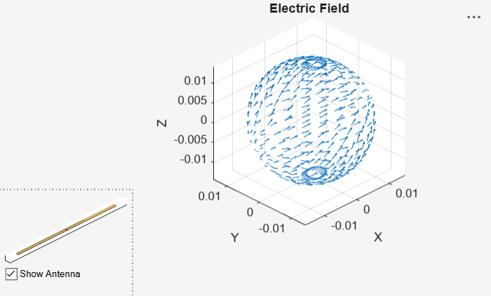

Create a measuredAntenna object and set its properties using the electric field data, spherical coordinates of the observation points, and the phase center. Assume the phase center location at 5λ along the z‑axis.

ms = measuredAntenna;
ms.E = E';
ms.Direction = [PHI(:), ELE(:), r*ones(numel(PHI),1)];
ms.FieldFrequency = freq;
ms.PhaseCenter = [0 0 5*lambda];

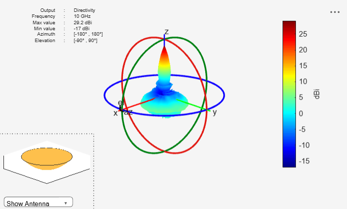
Create a parabolic reflector antenna with the measuredAntenna as its exciter. Plot the radiation pattern of this antenna at 10 GHz.

back = reflectorParabolic;
back.Exciter = ms;
figure
pattern(back,freq)

Import and Visualize Measured Radiation Pattern Data

Import the pattern data of a linear array of dipoles from a text file using the readmatrix function. Define the frequency range for the data and number of antenna elements in the array.

The text file contains measured field data at 1.6 GHz, 2 GHz, and 2.4 GHz frequencies.

fRange = [1.6e9 2e9 2.4e9];
numAnt = 2;
patternData = readmatrix("MeasuredData.txt");
patternData

patternData = 2701×30 complex
102 ×

   0.0000 - 0.0000i   0.0000 + 0.0000i   0.0000 + 0.0000i  -0.0000 + 0.0000i   0.0000 - 0.0000i   0.0000 + 0.0000i  -0.0000 - 0.0000i   0.0000 - 0.0000i   0.0000 - 0.0000i  -1.8000 + 0.0000i  -0.9000 + 0.0000i   0.1500 + 0.0000i   0.0000 - 0.0000i   0.0000 + 0.0000i   0.0000 + 0.0000i  -0.0000 + 0.0000i   0.0000 + 0.0000i   0.0000 + 0.0000i  -0.0000 - 0.0000i   0.0000 - 0.0000i   0.0000 + 0.0000i   0.0000 + 0.0000i   0.0000 - 0.0000i   0.0000 + 0.0000i  -0.0000 - 0.0000i   0.0000 - 0.0000i   0.0000 - 0.0000i   0.0000 + 0.0000i   0.0000 - 0.0000i   0.0000 - 0.0000i
   0.0000 - 0.0000i   0.0000 + 0.0000i   0.0000 + 0.0000i  -0.0000 + 0.0000i   0.0000 - 0.0000i   0.0000 + 0.0000i  -0.0000 - 0.0000i   0.0000 - 0.0000i   0.0000 - 0.0000i  -1.7500 + 0.0000i  -0.9000 + 0.0000i   0.1500 + 0.0000i   0.0000 - 0.0000i   0.0000 + 0.0000i   0.0000 + 0.0000i  -0.0000 + 0.0000i   0.0000 + 0.0000i   0.0000 + 0.0000i  -0.0000 - 0.0000i   0.0000 - 0.0000i   0.0000 + 0.0000i   0.0000 + 0.0000i   0.0000 - 0.0000i   0.0000 + 0.0000i  -0.0000 - 0.0000i   0.0000 - 0.0000i   0.0000 - 0.0000i   0.0000 + 0.0000i   0.0000 - 0.0000i   0.0000 - 0.0000i
   0.0000 - 0.0000i   0.0000 + 0.0000i   0.0000 + 0.0000i  -0.0000 + 0.0000i   0.0000 - 0.0000i   0.0000 + 0.0000i  -0.0000 - 0.0000i   0.0000 - 0.0000i   0.0000 - 0.0000i  -1.7000 + 0.0000i  -0.9000 + 0.0000i   0.1500 + 0.0000i   0.0000 - 0.0000i   0.0000 + 0.0000i   0.0000 + 0.0000i  -0.0000 + 0.0000i   0.0000 + 0.0000i   0.0000 + 0.0000i  -0.0000 - 0.0000i   0.0000 - 0.0000i   0.0000 + 0.0000i   0.0000 + 0.0000i   0.0000 - 0.0000i   0.0000 + 0.0000i  -0.0000 - 0.0000i   0.0000 - 0.0000i   0.0000 - 0.0000i   0.0000 + 0.0000i   0.0000 - 0.0000i   0.0000 - 0.0000i
   0.0000 - 0.0000i   0.0000 + 0.0000i   0.0000 + 0.0000i  -0.0000 + 0.0000i   0.0000 - 0.0000i   0.0000 + 0.0000i  -0.0000 - 0.0000i   0.0000 - 0.0000i   0.0000 - 0.0000i  -1.6500 + 0.0000i  -0.9000 + 0.0000i   0.1500 + 0.0000i   0.0000 - 0.0000i   0.0000 + 0.0000i   0.0000 + 0.0000i  -0.0000 + 0.0000i   0.0000 + 0.0000i   0.0000 + 0.0000i  -0.0000 - 0.0000i   0.0000 - 0.0000i   0.0000 + 0.0000i   0.0000 + 0.0000i   0.0000 - 0.0000i   0.0000 + 0.0000i  -0.0000 - 0.0000i   0.0000 - 0.0000i   0.0000 - 0.0000i   0.0000 + 0.0000i   0.0000 - 0.0000i   0.0000 - 0.0000i
   0.0000 - 0.0000i   0.0000 + 0.0000i   0.0000 + 0.0000i  -0.0000 + 0.0000i   0.0000 - 0.0000i   0.0000 + 0.0000i  -0.0000 - 0.0000i   0.0000 - 0.0000i   0.0000 - 0.0000i  -1.6000 + 0.0000i  -0.9000 + 0.0000i   0.1500 + 0.0000i   0.0000 - 0.0000i   0.0000 + 0.0000i   0.0000 + 0.0000i  -0.0000 + 0.0000i   0.0000 + 0.0000i   0.0000 + 0.0000i  -0.0000 - 0.0000i   0.0000 - 0.0000i   0.0000 + 0.0000i   0.0000 + 0.0000i   0.0000 - 0.0000i   0.0000 + 0.0000i  -0.0000 - 0.0000i   0.0000 - 0.0000i   0.0000 - 0.0000i   0.0000 + 0.0000i   0.0000 - 0.0000i   0.0000 - 0.0000i
   0.0000 - 0.0000i   0.0000 + 0.0000i   0.0000 + 0.0000i  -0.0000 + 0.0000i   0.0000 - 0.0000i   0.0000 + 0.0000i  -0.0000 - 0.0000i   0.0000 - 0.0000i   0.0000 - 0.0000i  -1.5500 + 0.0000i  -0.9000 + 0.0000i   0.1500 + 0.0000i   0.0000 - 0.0000i   0.0000 + 0.0000i   0.0000 + 0.0000i  -0.0000 + 0.0000i   0.0000 + 0.0000i   0.0000 + 0.0000i  -0.0000 - 0.0000i   0.0000 - 0.0000i   0.0000 + 0.0000i   0.0000 + 0.0000i   0.0000 - 0.0000i   0.0000 + 0.0000i  -0.0000 - 0.0000i   0.0000 - 0.0000i   0.0000 - 0.0000i   0.0000 + 0.0000i   0.0000 - 0.0000i   0.0000 - 0.0000i
   0.0000 - 0.0000i   0.0000 + 0.0000i   0.0000 + 0.0000i  -0.0000 + 0.0000i   0.0000 - 0.0000i   0.0000 + 0.0000i  -0.0000 - 0.0000i   0.0000 - 0.0000i   0.0000 - 0.0000i  -1.5000 + 0.0000i  -0.9000 + 0.0000i   0.1500 + 0.0000i   0.0000 - 0.0000i   0.0000 + 0.0000i   0.0000 + 0.0000i  -0.0000 + 0.0000i   0.0000 + 0.0000i   0.0000 + 0.0000i  -0.0000 - 0.0000i   0.0000 - 0.0000i   0.0000 + 0.0000i   0.0000 + 0.0000i   0.0000 - 0.0000i   0.0000 + 0.0000i  -0.0000 - 0.0000i   0.0000 - 0.0000i   0.0000 - 0.0000i   0.0000 + 0.0000i   0.0000 - 0.0000i   0.0000 - 0.0000i
   0.0000 - 0.0000i   0.0000 + 0.0000i   0.0000 + 0.0000i  -0.0000 + 0.0000i   0.0000 - 0.0000i   0.0000 + 0.0000i  -0.0000 - 0.0000i   0.0000 - 0.0000i   0.0000 - 0.0000i  -1.4500 + 0.0000i  -0.9000 + 0.0000i   0.1500 + 0.0000i   0.0000 - 0.0000i   0.0000 + 0.0000i   0.0000 + 0.0000i  -0.0000 + 0.0000i   0.0000 + 0.0000i   0.0000 + 0.0000i  -0.0000 - 0.0000i   0.0000 - 0.0000i   0.0000 + 0.0000i   0.0000 + 0.0000i   0.0000 - 0.0000i   0.0000 + 0.0000i  -0.0000 - 0.0000i   0.0000 - 0.0000i   0.0000 - 0.0000i   0.0000 + 0.0000i   0.0000 - 0.0000i   0.0000 - 0.0000i
   0.0000 - 0.0000i   0.0000 + 0.0000i   0.0000 + 0.0000i  -0.0000 + 0.0000i   0.0000 - 0.0000i   0.0000 + 0.0000i  -0.0000 - 0.0000i   0.0000 - 0.0000i   0.0000 - 0.0000i  -1.4000 + 0.0000i  -0.9000 + 0.0000i   0.1500 + 0.0000i   0.0000 - 0.0000i   0.0000 + 0.0000i   0.0000 + 0.0000i  -0.0000 + 0.0000i   0.0000 + 0.0000i   0.0000 + 0.0000i  -0.0000 - 0.0000i   0.0000 - 0.0000i   0.0000 + 0.0000i   0.0000 + 0.0000i   0.0000 - 0.0000i   0.0000 + 0.0000i  -0.0000 - 0.0000i   0.0000 - 0.0000i   0.0000 - 0.0000i   0.0000 + 0.0000i   0.0000 - 0.0000i   0.0000 - 0.0000i
   0.0000 - 0.0000i   0.0000 + 0.0000i   0.0000 + 0.0000i  -0.0000 + 0.0000i   0.0000 - 0.0000i   0.0000 + 0.0000i  -0.0000 - 0.0000i   0.0000 - 0.0000i   0.0000 - 0.0000i  -1.3500 + 0.0000i  -0.9000 + 0.0000i   0.1500 + 0.0000i   0.0000 - 0.0000i   0.0000 + 0.0000i   0.0000 + 0.0000i  -0.0000 + 0.0000i   0.0000 + 0.0000i   0.0000 + 0.0000i  -0.0000 - 0.0000i   0.0000 - 0.0000i   0.0000 + 0.0000i   0.0000 + 0.0000i   0.0000 - 0.0000i   0.0000 + 0.0000i  -0.0000 - 0.0000i   0.0000 - 0.0000i   0.0000 - 0.0000i   0.0000 + 0.0000i   0.0000 - 0.0000i   0.0000 - 0.0000i
   0.0000 - 0.0000i   0.0000 + 0.0000i   0.0000 + 0.0000i  -0.0000 + 0.0000i   0.0000 - 0.0000i   0.0000 + 0.0000i  -0.0000 - 0.0000i   0.0000 - 0.0000i   0.0000 - 0.0000i  -1.3000 + 0.0000i  -0.9000 + 0.0000i   0.1500 + 0.0000i   0.0000 - 0.0000i   0.0000 + 0.0000i   0.0000 + 0.0000i  -0.0000 + 0.0000i   0.0000 + 0.0000i   0.0000 + 0.0000i  -0.0000 - 0.0000i   0.0000 - 0.0000i   0.0000 + 0.0000i   0.0000 + 0.0000i   0.0000 - 0.0000i   0.0000 + 0.0000i  -0.0000 - 0.0000i   0.0000 - 0.0000i   0.0000 - 0.0000i   0.0000 + 0.0000i   0.0000 - 0.0000i   0.0000 - 0.0000i
   0.0000 - 0.0000i   0.0000 + 0.0000i   0.0000 + 0.0000i  -0.0000 + 0.0000i   0.0000 - 0.0000i   0.0000 + 0.0000i  -0.0000 - 0.0000i   0.0000 - 0.0000i   0.0000 - 0.0000i  -1.2500 + 0.0000i  -0.9000 + 0.0000i   0.1500 + 0.0000i   0.0000 - 0.0000i   0.0000 + 0.0000i   0.0000 + 0.0000i  -0.0000 + 0.0000i   0.0000 + 0.0000i   0.0000 + 0.0000i  -0.0000 - 0.0000i   0.0000 - 0.0000i   0.0000 + 0.0000i   0.0000 + 0.0000i   0.0000 - 0.0000i   0.0000 + 0.0000i  -0.0000 - 0.0000i   0.0000 - 0.0000i   0.0000 - 0.0000i   0.0000 + 0.0000i   0.0000 - 0.0000i   0.0000 - 0.0000i
   0.0000 - 0.0000i   0.0000 + 0.0000i   0.0000 + 0.0000i  -0.0000 + 0.0000i   0.0000 - 0.0000i   0.0000 + 0.0000i  -0.0000 - 0.0000i   0.0000 - 0.0000i   0.0000 - 0.0000i  -1.2000 + 0.0000i  -0.9000 + 0.0000i   0.1500 + 0.0000i   0.0000 - 0.0000i   0.0000 + 0.0000i   0.0000 + 0.0000i  -0.0000 + 0.0000i   0.0000 + 0.0000i   0.0000 + 0.0000i  -0.0000 - 0.0000i   0.0000 - 0.0000i   0.0000 + 0.0000i   0.0000 + 0.0000i   0.0000 - 0.0000i   0.0000 + 0.0000i  -0.0000 - 0.0000i   0.0000 - 0.0000i   0.0000 - 0.0000i   0.0000 + 0.0000i   0.0000 - 0.0000i   0.0000 - 0.0000i
   0.0000 - 0.0000i   0.0000 + 0.0000i   0.0000 + 0.0000i  -0.0000 + 0.0000i   0.0000 - 0.0000i   0.0000 + 0.0000i  -0.0000 - 0.0000i   0.0000 - 0.0000i   0.0000 - 0.0000i  -1.1500 + 0.0000i  -0.9000 + 0.0000i   0.1500 + 0.0000i   0.0000 - 0.0000i   0.0000 + 0.0000i   0.0000 + 0.0000i  -0.0000 + 0.0000i   0.0000 + 0.0000i   0.0000 + 0.0000i  -0.0000 - 0.0000i   0.0000 - 0.0000i   0.0000 + 0.0000i   0.0000 + 0.0000i   0.0000 - 0.0000i   0.0000 + 0.0000i  -0.0000 - 0.0000i   0.0000 - 0.0000i   0.0000 - 0.0000i   0.0000 + 0.0000i   0.0000 - 0.0000i   0.0000 - 0.0000i
   0.0000 - 0.0000i   0.0000 + 0.0000i   0.0000 + 0.0000i  -0.0000 + 0.0000i   0.0000 - 0.0000i   0.0000 + 0.0000i  -0.0000 - 0.0000i   0.0000 - 0.0000i   0.0000 - 0.0000i  -1.1000 + 0.0000i  -0.9000 + 0.0000i   0.1500 + 0.0000i   0.0000 - 0.0000i   0.0000 + 0.0000i   0.0000 + 0.0000i  -0.0000 + 0.0000i   0.0000 + 0.0000i   0.0000 + 0.0000i  -0.0000 - 0.0000i   0.0000 - 0.0000i   0.0000 + 0.0000i   0.0000 + 0.0000i   0.0000 - 0.0000i   0.0000 + 0.0000i  -0.0000 - 0.0000i   0.0000 - 0.0000i   0.0000 - 0.0000i   0.0000 + 0.0000i   0.0000 - 0.0000i   0.0000 - 0.0000i
      ⋮

Extract the field data, direction data, and embedded field data from the imported data. Further, extract azimuth and elevation data from the direction data.

% E-field data
eField(:,:,1) = patternData(:,1:3);
eField(:,:,2) = patternData(:,4:6);
eField(:,:,3) = patternData(:,7:9);

% Direction, azimuth, and elevation data
dir = patternData(:,10:12);
az = dir(1:73,1);
el = dir(1:73:end,2);

% Embedded E-field data
embE(:,:,1,1) = patternData(:,13:15);
embE(:,:,2,1) = patternData(:,16:18);
embE(:,:,1,2) = patternData(:,19:21);
embE(:,:,2,2) = patternData(:,22:24);
embE(:,:,1,3) = patternData(:,25:27);
embE(:,:,2,3) = patternData(:,28:30);

Import and extract S-parameters data from Touchstone files.

% Import S-parameters data
sParamData1 = sparameters("Parameters_1.6ghz.s2p");
sParamData2 = sparameters("Parameters_2ghz.s2p");
sParamData3 = sparameters("Parameters_2.4ghz.s2p");

% Extract S-parameters data
sParam(:,:,1) = sParamData1.Parameters;
sParam(:,:,2) = sParamData2.Parameters;
sParam(:,:,3) = sParamData3.Parameters;
sParamFreq(:,1) = sParamData1.Frequencies;
sParamFreq(:,2) = sParamData2.Frequencies;
sParamFreq(:,3) = sParamData3.Frequencies;
sParam

sParam = 
sParam(:,:,1) =

   0.6991 - 0.5140i   0.0523 + 0.0366i
   0.0523 + 0.0366i   0.6991 - 0.5140i


sParam(:,:,2) =

   0.2076 - 0.0674i  -0.0918 - 0.1830i
  -0.0918 - 0.1830i   0.2076 - 0.0674i


sParam(:,:,3) =

   0.6581 + 0.2567i  -0.0490 + 0.0871i
  -0.0490 + 0.0871i   0.6581 + 0.2567i

sParamFreq

sParamFreq = 1×3
109 ×

    1.6000    2.0000    2.4000

s = sparameters(sParam,sParamFreq);

Create a measuredAntenna object and set its properties using the extracted data.

mesAnt = measuredAntenna(E=eField, Direction=dir, NumPorts=numAnt,...
    Azimuth=az, Elevation=el, FieldCoordinate="polar",...
    EmbeddedE=embE, FieldFrequency=fRange, Sparameters=s)

mesAnt = 
  measuredAntenna with properties:

                       E: [2701×3×3 double]
             Directivity: []
               Direction: [2701×3 double]
             PhaseCenter: [0 0 0.0750]
                NumPorts: 2
          FieldFrequency: [3×1 double]
         FieldCoordinate: "polar"
                 Azimuth: [-180 -175 -170 -165 -160 -155 -150 -145 -140 -135 -130 -125 -120 -115 -110 -105 -100 -95 -90 -85 -80 -75 -70 -65 -60 -55 -50 -45 -40 -35 -30 -25 -20 -15 -10 -5 0 5 10 15 20 25 30 35 40 45 50 55 60 65 70 75 80 … ] (1×73 double)
               Elevation: [-90 -85 -80 -75 -70 -65 -60 -55 -50 -45 -40 -35 -30 -25 -20 -15 -10 -5 0 5 10 15 20 25 30 35 40 45 50 55 60 65 70 75 80 85 90]
             Sparameters: [1×1 sparameters]
          AmplitudeTaper: 1
              PhaseShift: 0
               EmbeddedE: [2701×3×2×3 double]
    TerminationImpedance: 50
     CalculateTotalField: 0

Visualize Measured Pattern Data

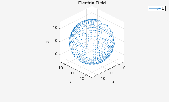
Plot the radiation pattern and electric field for this measuredAntenna at 2 GHz, while plot S-parameters over the entire frequency range.

pattern(mesAnt,fRange(2),Type="efield")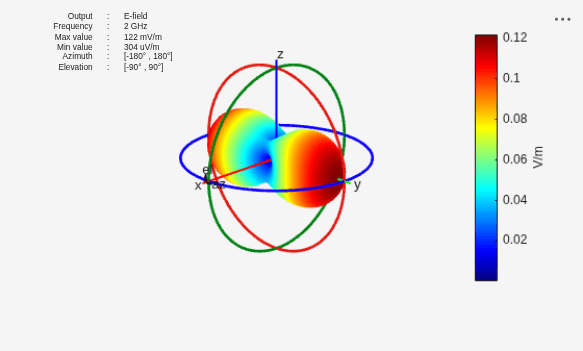

EHfields(mesAnt,fRange(2))

sp = sparameters(mesAnt,fRange);
rfplot(sp)

Import and Visualize Radiation Pattern Data from FFD File

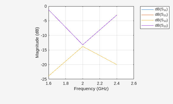
The .ffd file contains far-field data generated by the HFSS™ software. Load the radiation pattern data from the .ffd file into the workspace by using the loadData helper function defined in the Supporting Function section of this example. Specify the coordinate system angle convention used for this data in the .ffd file.

fileName = sprintf("RefFFDdata.ffd");
CoordinateSystem = "Phi-Theta";
[theta1,phi1,numFreqs,Etheta,Ephi,freqs] = loadData(fileName,CoordinateSystem);
if CoordinateSystem == "Phi-Theta"
    elev = 90 - theta1;
else
    elev = theta1;
end

Calculate the number of data points.

numPt = numel(theta1)*numel(phi1);

Extract the electric field data from the data in the workspace.

ESph = [Ephi;Etheta;zeros(numPt,3)];
eField = reshape(ESph,numPt,3,numFreqs);

Calculate the spherical coordinates of the electric field points.

lambda = 3e8/max(freqs);
radius = 100*lambda*ones(numPt,1);
[theta,phi] = meshgrid(elev,phi1);
phi = phi(:);
theta = theta(:);
direction = [phi theta radius];

Create a measuredAntenna object with the number of ports equal to those in the .ffd file data. Specify the E property using eField, and set the Direction property using calculated spherical coordinates. Set the Azimuth and Elevation properties using phi1 and elev, respectively. Specify the phase center. This example assumes the phase center at (0,0,0). Set the FieldFrequency property using the frequencies of the electric field data.

mAnt = measuredAntenna(NumPorts=1);
mAnt.E = eField;
mAnt.Direction = direction;
mAnt.PhaseCenter = [0 0 0];
mAnt.FieldFrequency = freqs;
mAnt.Azimuth = phi1;
mAnt.Elevation = elev;
mAnt.FieldCoordinate = 'polar';

Visualize the radiation patterns at the individual frequencies.

for i=1:numFreqs
figure
pattern(mAnt,freqs(i))
title(strcat("Radiation Pattern at ",num2str(freqs(i)/1e9)," GHz"))
end

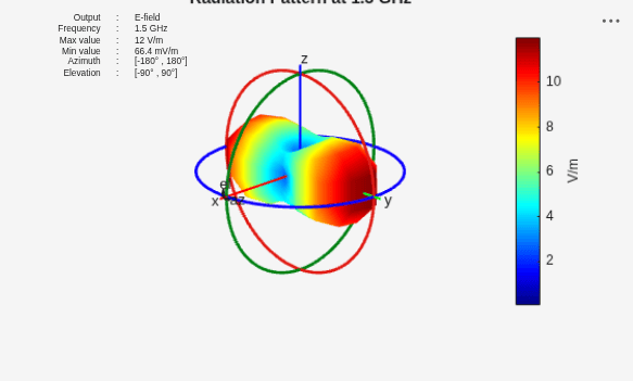
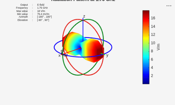
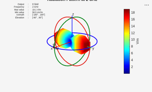
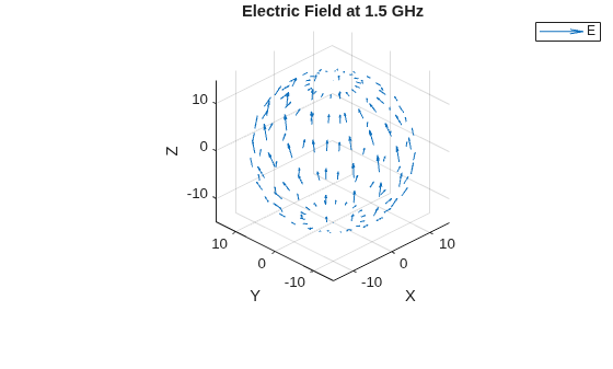
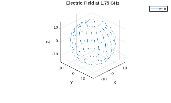
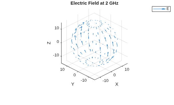
Visualize the corresponding electric fields.

for i=1:numFreqs
figure
EHfields(mAnt,freqs(i))
title(strcat("Electric Field at ",num2str(freqs(i)/1e9)," GHz"))
end

Supporting Function

The loadData helper function extracts the number of frequencies, angle values for the data points, and the electric field values from the .ffd file.

function [theta1,phi1,numFreqs,Etheta,Ephi,freqs] = loadData(fileName,CoordinateSystem)
fid = fopen(fileName);

if CoordinateSystem == "Phi-Theta"
    numHeaderLines = 3;
else
    textscan(fid,'%s',1);
    numHeaderLines = 4;
end

data = num2cell(fscanf(fid,'%d',3));
theta1 = linspace(data{:});
data = num2cell(fscanf(fid,'%d',3));
phi1 = linspace(data{:});
C1 = textscan(fid,'%s %d',1);
numFreqs = C1{2};
fclose(fid);

Mfull = readmatrix(fileName,FileType="text",NumHeaderLines=numHeaderLines);
freqs = Mfull(isnan(Mfull(:,1)),2);
MData = Mfull(~isnan(Mfull(:,1)),:);
Etheta = reshape(MData(:,1) + 1j*MData(:,2),length(phi1)*length(theta1),[]);
Ephi = reshape(MData(:,3) + 1j*MData(:,4),length(phi1)*length(theta1),[]);
end

Perform Pattern Multiplication for Rectangular Array Using Measured Element Pattern Data

Load the measured E-field data. Define the field frequency, azimuth, and elevation angles.

load("mesAnt_rect_array.mat")
freq = 3e9;
az = -180:5:180;
el = -90:5:90;

Create a measuredAntenna object and set its properties using the defined parameters.

mesAnt = measuredAntenna(E=Efield,Direction=Dir,NumPorts=1, ...
    Azimuth=az,Elevation=el,FieldCoordinate="rectangular", ...
    FieldFrequency=freq)

mesAnt = 
  measuredAntenna with properties:

                  E: [2701×3 double]
        Directivity: []
          Direction: [2701×3 double]
        PhaseCenter: [0 0 0.0750]
           NumPorts: 1
     FieldFrequency: 3.0000e+09
    FieldCoordinate: "rectangular"
            Azimuth: [-180 -175 -170 -165 -160 -155 -150 -145 -140 -135 -130 -125 -120 -115 -110 -105 -100 -95 -90 -85 -80 -75 -70 -65 -60 -55 -50 -45 -40 -35 -30 -25 -20 -15 -10 -5 0 5 10 15 20 25 30 35 40 45 50 55 60 65 70 75 80 85 90 … ] (1×73 double)
          Elevation: [-90 -85 -80 -75 -70 -65 -60 -55 -50 -45 -40 -35 -30 -25 -20 -15 -10 -5 0 5 10 15 20 25 30 35 40 45 50 55 60 65 70 75 80 85 90]
        Sparameters: []

Create a 2-by-2 rectangular array with 0.0665 m row and column spacing and use the measuredAntenna object as its element.

rectArr = rectangularArray(Element=mesAnt,RowSpacing=0.0665,ColumnSpacing=0.0665)

rectArr = 
  rectangularArray with properties:

           Element: [1×1 measuredAntenna]
              Size: [2 2]
        RowSpacing: 0.0665
     ColumnSpacing: 0.0665
           Lattice: 'Rectangular'
    AmplitudeTaper: 1
        PhaseShift: 0
              Tilt: 0
          TiltAxis: [1 0 0]

Perform pattern multiplication and plot the resultant array directivity pattern.

figure 
patternMultiply(rectArr,freq)

Integrate Reconstructed 3-D Pattern from Vertical and Horizontal Slices

Import horizontal and vertical slice directivity data of a dipole antenna operating at 75 MHz. This data includes magnitude, phi, and theta values at an angular resolution of 5 degrees.

load("slices_data.mat");

Reconstruct 3-D pattern of the antenna from the horizontal and vertical slices.

[patS,thout,phiout] = patternFromSlices(vertSlice,theta,horizSlice,phi,Method="CrossWeighted");

Calculate azimuth and elevation values.

frequency = 75e6;
lambda = physconst("LightSpeed")/frequency;
R = 100*lambda;
[az,el] = meshgrid(phiout,90-thout);
Dir = [az(:) el(:) R*ones(numel(az),1)];

Create a measuredAntenna object and set its properties. You can integrate this object into your workflow.

mAnt = measuredAntenna(E=[],Directivity=patS(:),Direction=Dir, ...
    FieldFrequency=frequency,FieldCoordinate="polar", ...
    PhaseCenter=[0 0 0],Azimuth=phiout,Elevation=90-thout);

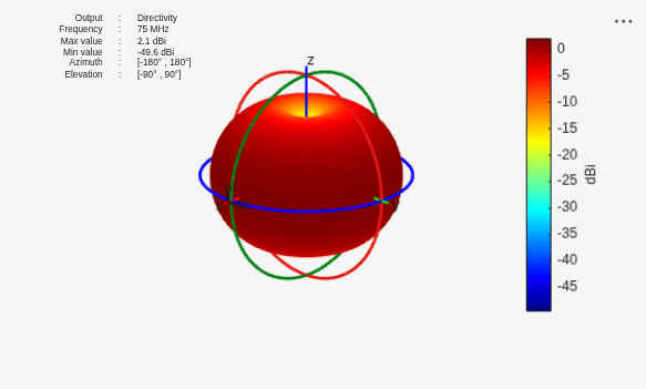
Compute pattern with default resolution.

figure
pattern(mAnt,frequency)

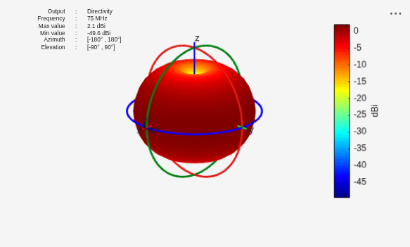
Compute pattern with lower resolution.

figure
pattern(mAnt,frequency,-180:15:180,-90:10:90)

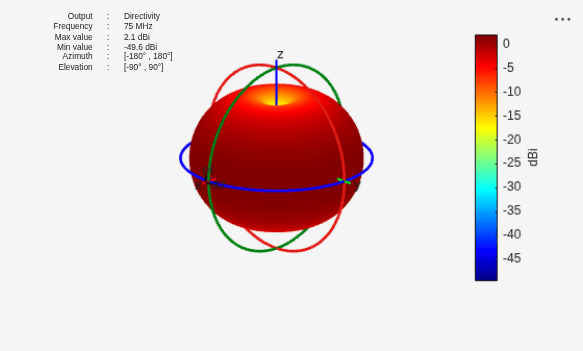
Compute pattern with higher resolution.

figure
pattern(mAnt,frequency,-180:1:180,-90:1:90)

Import and Plot Pattern Data with Multiple Frequencies

Load the file containing pattern data into the workspace. Define frequencies, azimuth, and elevation ranges for the data.

load("pattern_data.mat")
freq = 70e6:10e6:100e6;

Calculate directions for the pattern data. Create a measuredAntenna object and set its properties using the pattern data.

lambda = physconst("LightSpeed")/70e6;
R = 100*lambda;
[az1, el1] = meshgrid(az,el);

Dir = [az1(:) el1(:) R*ones(numel(az1),1)];

mAnt = measuredAntenna(E=[],Directivity=patT,Direction=Dir,FieldFrequency=freq, ...
    Azimuth=az,Elevation=el,PhaseCenter=[0 0 0]);

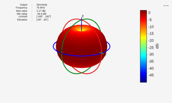
Calculate and plot the directivity pattern at 75 MHz. The measuredAntenna object interpolates pattern data for the frequencies, azimuth, and elevation angles that are within the specified range.

[mPat,mAz,mEl] = pattern(mAnt,75e6,-180:25:180,-90:20:90)

mPat = 10×15

  -49.9273  -49.9273  -49.9273  -49.9273  -49.9273  -49.9273  -49.9273  -49.9273  -49.9273  -49.9273  -49.9273  -49.9273  -49.9273  -49.9273  -49.9273
   -9.2430   -9.2447   -9.2458   -9.2464   -9.2465   -9.2460   -9.2450   -9.2434   -9.2415   -9.2396   -9.2383   -9.2380   -9.2387   -9.2403   -9.2423
   -3.0441   -3.0446   -3.0449   -3.0452   -3.0452   -3.0450   -3.0447   -3.0442   -3.0438   -3.0435   -3.0432   -3.0432   -3.0433   -3.0436   -3.0440
    0.3401    0.3399    0.3395    0.3391    0.3391    0.3394    0.3398    0.3401    0.3400    0.3396    0.3393    0.3392    0.3394    0.3398    0.3401
    1.9635    1.9632    1.9626    1.9621    1.9620    1.9625    1.9631    1.9635    1.9633    1.9626    1.9620    1.9619    1.9622    1.9629    1.9634
    1.9635    1.9632    1.9625    1.9620    1.9619    1.9624    1.9631    1.9635    1.9633    1.9627    1.9621    1.9620    1.9623    1.9630    1.9634
    0.3401    0.3399    0.3396    0.3392    0.3392    0.3395    0.3399    0.3401    0.3399    0.3395    0.3392    0.3391    0.3393    0.3397    0.3400
   -3.0441   -3.0437   -3.0434   -3.0432   -3.0432   -3.0433   -3.0437   -3.0441   -3.0445   -3.0449   -3.0451   -3.0452   -3.0451   -3.0447   -3.0443
   -9.2430   -9.2411   -9.2393   -9.2382   -9.2381   -9.2390   -9.2407   -9.2426   -9.2444   -9.2457   -9.2463   -9.2465   -9.2461   -9.2452   -9.2437
  -49.9273  -49.9273  -49.9273  -49.9273  -49.9273  -49.9273  -49.9273  -49.9273  -49.9273  -49.9273  -49.9273  -49.9273  -49.9273  -49.9273  -49.9273

mAz = 1×15

  -180  -155  -130  -105   -80   -55   -30    -5    20    45    70    95   120   145   170

mEl = 1×10

   -90   -70   -50   -30   -10    10    30    50    70    90

figure
pattern(mAnt,75e6)

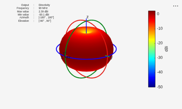
Calculate and plot the directivity pattern at 90 MHz.

[mPat1,mAz1,mEl1] = pattern(mAnt,90e6,-180:25:180,-90:20:90)

mPat1 = 10×15

  -50.0580  -50.0580  -50.0580  -50.0580  -50.0580  -50.0580  -50.0580  -50.0580  -50.0580  -50.0580  -50.0580  -50.0580  -50.0580  -50.0580  -50.0580
  -10.2357  -10.2503  -10.2619  -10.2685  -10.2691  -10.2636  -10.2529  -10.2388  -10.2237  -10.2106  -10.2021  -10.2001  -10.2048  -10.2154  -10.2296
   -3.5977   -3.6030   -3.6073   -3.6098   -3.6101   -3.6080   -3.6040   -3.5988   -3.5935   -3.5889   -3.5861   -3.5854   -3.5870   -3.5906   -3.5955
    0.2452    0.2430    0.2408    0.2393    0.2392    0.2404    0.2425    0.2448    0.2467    0.2479    0.2485    0.2486    0.2483    0.2475    0.2460
    2.1480    2.1471    2.1457    2.1447    2.1446    2.1455    2.1468    2.1479    2.1481    2.1477    2.1472    2.1470    2.1474    2.1480    2.1481
    2.1480    2.1481    2.1476    2.1471    2.1470    2.1475    2.1480    2.1481    2.1473    2.1460    2.1448    2.1445    2.1452    2.1465    2.1477
    0.2452    0.2470    0.2481    0.2486    0.2486    0.2482    0.2473    0.2456    0.2434    0.2412    0.2395    0.2391    0.2401    0.2420    0.2444
   -3.5977   -3.5925   -3.5882   -3.5857   -3.5855   -3.5876   -3.5915   -3.5966   -3.6020   -3.6066   -3.6095   -3.6102   -3.6086   -3.6049   -3.5999
  -10.2357  -10.2208  -10.2085  -10.2012  -10.2005  -10.2065  -10.2181  -10.2327  -10.2475  -10.2599  -10.2676  -10.2695  -10.2652  -10.2554  -10.2418
  -50.0580  -50.0580  -50.0580  -50.0580  -50.0580  -50.0580  -50.0580  -50.0580  -50.0580  -50.0580  -50.0580  -50.0580  -50.0580  -50.0580  -50.0580

mAz1 = 1×15

  -180  -155  -130  -105   -80   -55   -30    -5    20    45    70    95   120   145   170

mEl1 = 1×10

   -90   -70   -50   -30   -10    10    30    50    70    90

figure
pattern(mAnt,90e6)

Create RF Sites Using Pattern Data

Load the pattern data file into the workspace. Define the frequency for the pattern data and calculate directions. Create a measuredAntenna object and set its properties using the imported pattern data.

load("rf_site_data.mat");
frequency = 2.5e9;
lambda = physconst("LightSpeed")/frequency;
R = 100*lambda;
[az1, el1] = meshgrid(az,el);
Dir = [az1(:) el1(:) R*ones(numel(az1),1)];
mAnt = measuredAntenna(E=[],Directivity=pat(:),Direction=Dir,FieldFrequency=frequency, ...
    Azimuth=az,Elevation=el,PhaseCenter=[0 0 0]);

Create a site viewer, and Tx and Rx sites with their Antenna property specified using the measuredAntenna object.

viewer = siteviewer(Buildings="chicago.osm");

Warning: Unable to access basemap 'satellite', which uses an online source. Using 'darkwater' instead. More details: The connection to the URL 'https://services.arcgisonline.com/ArcGIS/rest/services/World_Imagery/MapServer' timed out.

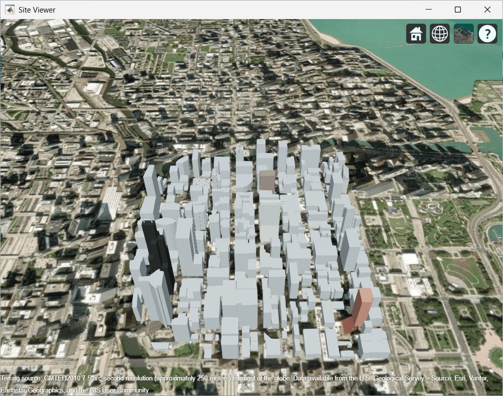
tx = txsite(Latitude=41.8800, ...
    Longitude=-87.6295, ...
    TransmitterFrequency=2.5e9,Antenna=mAnt);

rx = rxsite(Latitude=41.881352, ...
    Longitude=-87.629771, ...
    AntennaHeight=30,Antenna=mAnt);

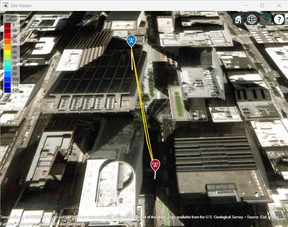
Use the raytracing propagation model to calculate the signal strength and perform raytracing.

pm = propagationModel("raytracing");
ss = sigstrength(rx,tx,pm)

ss = 
-50.0058

raytrace(tx,rx,pm)

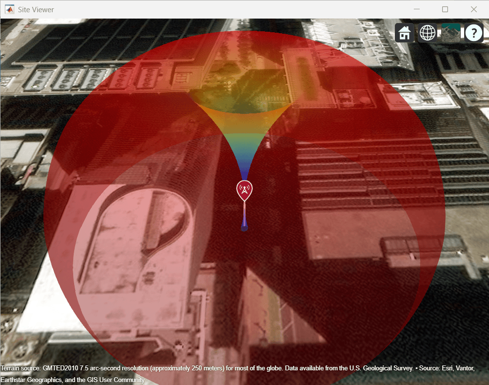
Plot the radiation pattern of the transmitter.

pattern(tx)

Integrate Pattern Data into Satellite Transmitter

Create the satelliteScenario object.

startTime = datetime(2020,11,25,0,0,0);
stopTime = startTime + days(1);
sampleTime = 60;
sc = satelliteScenario(startTime,stopTime,sampleTime);

Create the Satellite object. Create the Gimbal object for the satellite scenario using the Satellite object.

semiMajorAxis = 10000000;                                 % meters
eccentricity = 0;
inclination = 60;                                         % degrees
rightAscensionOfAscendingNode = 0;                        % degrees
argumentOfPeriapsis = 0;                                  % degrees
trueAnomaly = 0;                                          % degrees
sat = satellite(sc,semiMajorAxis,eccentricity,inclination, ...
    rightAscensionOfAscendingNode,argumentOfPeriapsis, ...
    trueAnomaly,Name="Satellite");
gimbaltxSat = gimbal(sat);

Specify parameters for the Transmitter object.

frequency = 27e9;                                    % Hz
power = 20;                                          % dBW
bitRate = 20;                                        % Mbps
systemLoss = 3;                                      % dB

Load the pattern data file into the workspace. Calculate the directions. Create a measuredAntenna object and set its properties using the imported pattern data.

load("ant_sat_data.mat");
lambda = physconst("LightSpeed")/frequency;
R = 100*lambda;
[az1, el1] = meshgrid(az,el);

Dir = [az1(:) el1(:) R*ones(numel(az1),1)];

mAnt = measuredAntenna(E=[],Directivity=pat(:),Direction=Dir, ...
    FieldFrequency=frequency,Azimuth=az,Elevation=el);

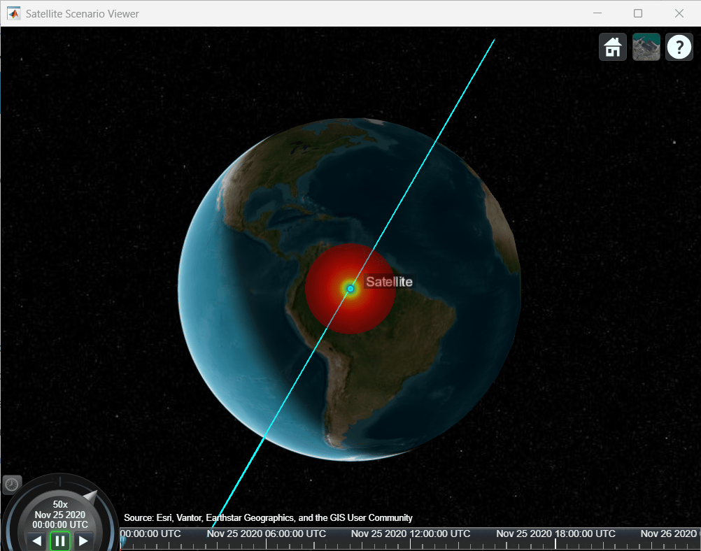
Create a Transmitter object. View the antenna radiation pattern in the scenario.

txSat = transmitter(gimbaltxSat,Name="Satellite Transmitter",Frequency=frequency, ...
    Power=power,BitRate=bitRate,SystemLoss=systemLoss,Antenna=mAnt);
viewer = satelliteScenarioViewer(sc);
pattern(txSat);

Use Measured Antenna Object in Antenna Block

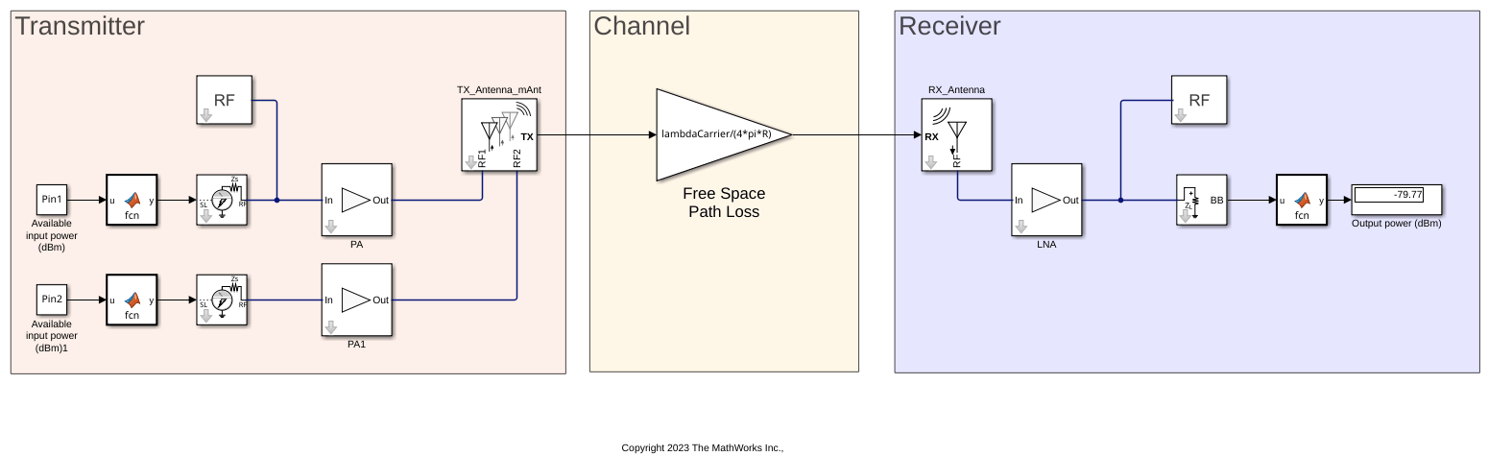
This example shows how to use measuredAntenna object in the Antenna block to model a measured antenna or array characterized by means of its S-parameters and frequency dependent far-field radiation pattern including both polarization components. The measuredAntenna object lets you replace the physical antennas from the antenna catalog with measured field data of the antenna. This example extracts data from a linear array to create a measuredAntenna object using hcreate_mAnt helper function.

System Configuration

Define the carrier frequency in Hz and set it in these parameters:

• Radiated carrier frequency parameter in the Transmit Antenna block

• Incident carrier frequency parameter in the Receiver Antenna block

• Carrier frequencies parameter in the Inport and Outport blocks

FreqCarrier = 5e9;

Define gain for the Gain block. This Gain block acts as a free-space path-loss channel.

lambdaCarrier = physconst('lightspeed')/FreqCarrier; %[m]

Define the input impedance of the low noise amplifier (LNA) in ohms.

Zin_r =71.3819 - 1j*2.1795;

Define the available input power in dBm for the two RF transmitter chains and assign the variables to Pin 1 and Pin 2 in the Constant block.

Pin1 = -30;
Pin2 = -30;

Create a linear antenna array and extract data from it to create a measuredAntenna object. The data extracted from the linear array is a substitute of real-world measured data that can be inputted by changing the hcreate_mAnt helper function so as to read the embedded electric fields from data file.

dist = lambdaCarrier*0.5;
d1 = design(dipole,FreqCarrier);
antElems = [d1 copy(d1)];
la = linearArray('Element',antElems,'ElementSpacing',dist);
la.TiltAxis = [0 1 0];
la.Tilt = 90;
freqRange = (4.5:0.05:5.5)*1e9;
[mAnt,R] = hcreate_mAnt(la,freqRange);

Compute impedances in ohms for PA and PA1 Amplifier blocks in the transmitter.

z = impedance(la,freqRange);
z = z(freqRange==FreqCarrier,:);
Zin_t1 = z(1);
Zin_t2 = z(2);

Simulate Model

Open and simulate the measuredAnt.slx model. Observe the output power at the receiver.

open_system("measuredAnt.slx")
sim("measuredAnt.slx");

Analyze Grating Lobes of Uniform Linear Array (ULA) Using E-field Data

Since R2026b

Import the field data of a circular microstrip patch antenna operating at 10 GHz.

load("field_data.mat")
freq = 10e9;
c = physconst("LightSpeed");
lambda = c/freq;

Create a measuredAntenna object and set its properties using this data.

mesAnt = measuredAntenna(E=Etotal,...
    Direction=Dir,...
    Azimuth=az,...
    Elevation=el,...
    FieldFrequency=freq,...
    PhaseCenter=[0 0 0],...
    NumPorts=1);

Create an ULA with measuredAntenna as its element.

numElements_ULA = 8;
elementSpacing_ULA = lambda/2;
ula = phased.ULA(NumElements=numElements_ULA,...
    ElementSpacing=elementSpacing_ULA,...
    Element=mesAnt,...
    ArrayAxis="y");

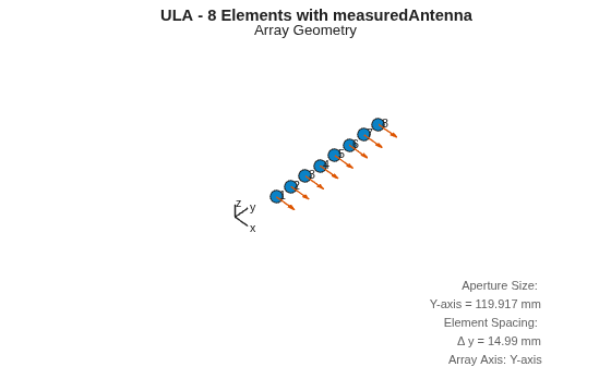
View the array geometry.

figure(Name="ULA Geometry");
viewArray(ula,ShowNormals=true,ShowIndex="All");
title("ULA - 8 Elements with measuredAntenna");

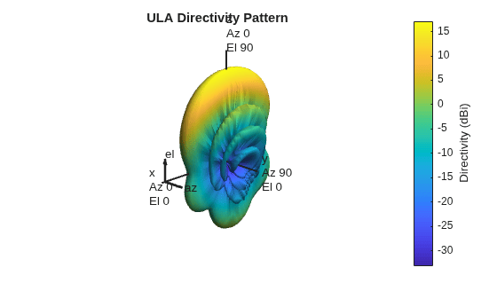
Plot 3-D directivity pattern of the array.

figure;
pattern(ula,freq,Type="directivity");
title("ULA Directivity Pattern");

For grating lobe analysis, create an array with a larger element spacing.

spacing_small = elementSpacing_ULA;
spacing_large = 2*elementSpacing_ULA;
ula_large = phased.ULA(NumElements=numElements_ULA,ElementSpacing=spacing_large,Element=mesAnt,ArrayAxis="y");

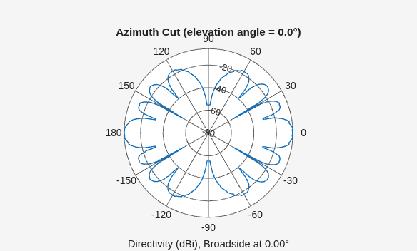
Plot the grating lobe diagram and azimuth pattern for the array with λ/2 element spacing. For half-wavelength spacing, the array satisfies the spatial sampling criterion and does not exhibit grating lobes in the visible region.

figure
plotGratingLobeDiagram(ula,freq,0);
title(sprintf("λ/2 Spacing (%.3f m)",spacing_small));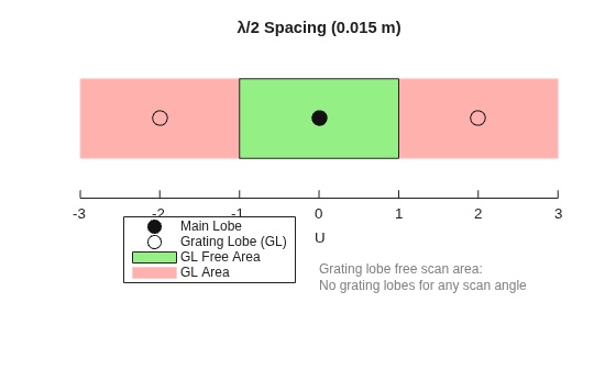

figure
patternAzimuth(ula,freq,0);

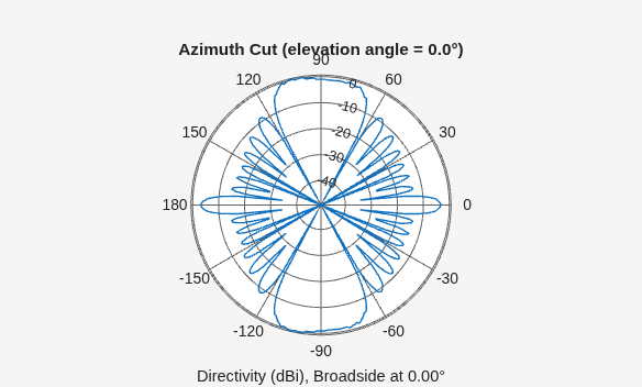
Plot the grating lobe diagram and azimuth pattern for the array with λ element spacing. When the element spacing is increased to one wavelength, additional lobes appear due to spatial aliasing. These grating lobes are visible both in the grating-lobe diagram and in the azimuth radiation pattern.

figure
plotGratingLobeDiagram(ula_large,freq,0);
title(sprintf("λ Spacing (%.3f m)",spacing_large));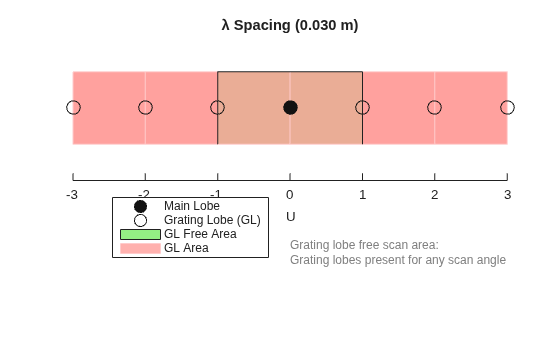

figure
patternAzimuth(ula_large,freq,0);

Beam Steering Using Antenna E-field Data

Since R2026b

Import the field data of a circular microstrip patch antenna operating at 10 GHz.

load("field_data.mat")
freq = 10e9;
c = physconst("LightSpeed");
lambda = c/freq;

Create a measuredAntenna object and set its properties using this data.

mesAnt = measuredAntenna(E=Etotal,...
    Direction=Dir,...
    Azimuth=az,...
    Elevation=el,...
    FieldFrequency=freq,...
    PhaseCenter=[0 0 0],...
    NumPorts=1);

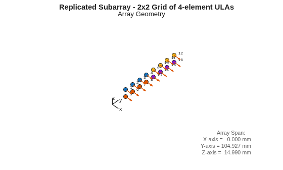
Create an uniform linear array (ULA) using the antenna field data. Use this ULA to create a 2-by-2 replicated subarray.

subarrayElement = phased.ULA(NumElements=4,ElementSpacing=lambda/2,Element=mesAnt);
numSubarrays = 4;
subarraySpacing = 2*lambda;

repSubarray = phased.ReplicatedSubarray(Subarray=subarrayElement,...
    Layout="Rectangular",...
    GridSize=[2, 2],...
    GridSpacing="Auto",...
    SubarraySteering="Phase");

Visualize the array geometry.

figure(Name="Replicated Subarray Geometry");
viewArray(repSubarray,ShowNormals=true,ShowIndex="All");
title("Replicated Subarray - 2x2 Grid of 4-element ULAs");

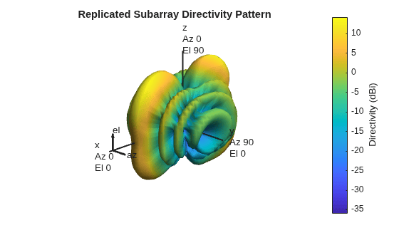
Plot 3-D directivity pattern of the array.

figure(Name="Replicated Subarray - 3D Pattern");
pattern(repSubarray,freq,Type="directivity");
title("Replicated Subarray Directivity Pattern");

Steer the beam to 40° azimuth using the phased.SteeringVector System object™.

steeringAngle = [40; 0];
sv = phased.SteeringVector(SensorArray=repSubarray,PropagationSpeed=3e8);
weights = step(sv,freq,steeringAngle);

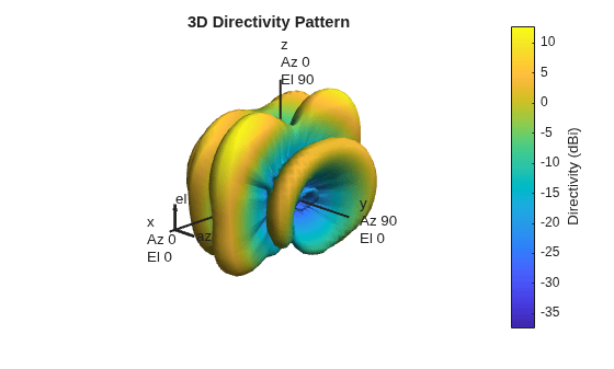
Plot the steered directivity pattern.

figure(Name="Replicated Subarray - Steered Pattern");
pattern(repSubarray,freq,Type="directivity",Weights=weights,...
    CoordinateSystem="polar")

Version History

Introduced in R2023a

R2026a: Specify directivity values

Use the new Directivity property to specify measured antenna or array directivity values.

R2024a: Calculate total electric field using embedded field data

Calculate the total electric field of an array from the embedded field, excitation amplitude, and phase shift of the individual antenna elements in the array. Use this calculated total electric field in the field analysis of the array using the pattern and EHfields functions.

R2023b: Perform field and port analysis on measured field data

Perform field and port analysis using pattern, EHfields, and sparameters on:

• The electric field and S-parameters data of an antenna

• The total electric field, embedded electric field, and S-parameters data of an array

measured at multiple frequencies.