Analyzing Affymetrix SNP Arrays for DNA Copy Number Variants

Open Script

This example shows how to study DNA copy number variants by preprocessing and analyzing data from the Affymetrix® GeneChip® Human Mapping 100k array.

Introduction

A copy number variant (CNV) is defined as a chromosomal segment that is 1kb or larger in length, whose copy number varies in comparison to a reference genome. CNV is one of the hallmarks of genetic instability common to most human cancers. When studying cancers, an important goal is to quickly and precisely identify copy number amplifications and deletions, and to assess their frequencies at the genome level. Recently, single nucleotide polymorphism (SNP) arrays have been used to detect and quantify genome-wide copy number alterations with high resolution. SNP array approaches also provide genotype information. For example, they can reveal loss of heterozygosity (LOH), which can provide supporting evidence for the presence of a deletion.

The Affymetrix GeneChip Mapping Array Set is a popular platform for high-throughput SNP genotyping and CNV detection. In this example, we use a publicly available data set from the Affymetrix 100K SNP array that interrogates over 100,000 SNP sites. You will import and preprocess the probe level data, estimate the raw signal ratios of the samples compared to references, and then infer copy numbers at each SNP locus after segmentation.

Data

Zhao et al. studied genome-wide copy number alterations of human lung carcinoma cell lines and primary tumors [1]. The samples were hybridized to Affymetrix 100K SNP arrays, each containing 115,593 mapped SNP loci. For this example, you will analyze data from 24 small cell lung carcinoma (SCLC) samples, of which 19 were primary tumor samples and 5 were cell line samples.

For each sample, SNPs were genotyped with two different arrays, Early Access 50KXba and Early Access 50KHind, in parallel. In brief, two aliquots of DNA samples were first digested with an XbaI or HindIII restriction enzyme, respectively. The digested DNA was ligated to an adaptor before subsequent polymerase chain reaction (PCR) amplification. Four PCR reactions were set up for each XbaI or HindIII adaptor-ligated DNA sample. The PCR products from the four reactions were pooled, concentrated, and fragmented to a size range of 250 to 2,000 bp. Fragmented PCR products were then labeled, denatured, and hybridized to the arrays.

For this example, you will work with data from the EA 50KXba array. To analyze the data from EA 50KHind array just repeat the steps. The SNP array data are stored in CEL files with each CEL file containing data from one array.

Note: High density SNP microarray data analysis requires extended amounts of memory from the operating system; if you receive "Out of memory" errors when running this example, try increasing the virtual memory (or swap space) of your operating system or try setting the 3GB switch (32-bit Windows® XP only). For details, see Resolve “Out of Memory” Errors.

This example uses the 50KXba and 50KHind SNP array data sets (not included in the toolbox) from the Meyerson Laboratory at the Dana-Farber Cancer Institute. You may use any other dataset to perform similar analyses.

The CDF library files used for these two arrays are CentXbaAv2.cdf and CentHindAv2.cdf. You can obtain these files from Affymetrix Web Site.

Set the variable Xba_celPath with the path to the location you stored the Xba array CEL files, and the variable libPath with the path to the location of the CDF library file for the EA 50KXba SNP array. (These files are not distributed with Bioinformatics Toolbox™).

Xba_celPath = 'C:\Examples\affysnpcnvdemo\Xba_array';
libPath = 'C:\Examples\affysnpcnvdemo\LibFiles';

SCLC_Sample_CEL.txt, a file provided with the Bioinformatics Toolbox™ software, contains a list of the 24 CEL file names used for this example, and the samples (5 SCLC cell lines and 19 primary tumors) to which they belong. Load this data into two MATLAB® variables.

fid = fopen('SCLC_Sample_CEL.txt','r');
ftext = textscan(fid, '%q%q');
fclose(fid);
samples = ftext{1};
cels = ftext{2};
nSample = numel(samples)

nSample =

    24

Accessing SNP Array Probe-Level Data

The Affymetrix 50KXba SNP array has a density up to 50K SNP sites. Each SNP on the array is represented by a collection of probe quartets. A probe quartet consists of a set of probe pairs for both alleles (A and B) and for both forward and reverse strands (antisense and sense) for the SNP. Each probe pair consists a perfect match (PM) probe and a mismatch (MM) probe. The Bioinformatics Toolbox software provides functions to access the probe-level data.

The function affyread reads the CEL files and the CDF library files for Affymetrix SNP arrays.

Read the sixth CEL file of the EA 50KXba data into a MATLAB structure.

s_cel = affyread(fullfile(Xba_celPath, [cels{6} '.CEL']))

s_cel = 

  struct with fields:

                Name: 'S0168T.CEL'
            DataPath: 'C:\Examples\affysnpcnvdemo\Xba_array'
             LibPath: 'C:\Examples\affysnpcnvdemo\Xba_array'
        FullPathName: 'C:\Examples\affysnpcnvdemo\Xba_array\S0168T.CEL'
            ChipType: 'CentXbaAv2'
                Date: '01-Feb-2013 11:54:13'
         FileVersion: 3
           Algorithm: 'Percentile'
           AlgParams: 'Percentile:75;CellMargin:2;OutlierHigh:1.500;OutlierLow:1.004;AlgVersion:6.0;FixedCellSize:TRUE;FullFeatureWidth:5;FullFeatureHeight:5;IgnoreOutliersInShiftRows:FALSE;FeatureExtraction:TRUE;PoolWidthExtenstion:2;PoolHeightExtension:2;UseSubgrids:FALSE;RandomizePixels:FALSE;ErrorBasis:StdvMean;StdMult:1.000000'
        NumAlgParams: 16
          CellMargin: 2
                Rows: 1600
                Cols: 1600
           NumMasked: 0
         NumOutliers: 12478
           NumProbes: 2560000
          UpperLeftX: 222
          UpperLeftY: 236
         UpperRightX: 8410
         UpperRightY: 219
          LowerLeftX: 252
          LowerLeftY: 8426
         LowerRightX: 8440
         LowerRightY: 8410
    ProbeColumnNames: {8×1 cell}
              Probes: [2560000×8 single]

Read the CDF library file for the EA 50KXba array into a MATLAB structure.

s_cdf = affyread(fullfile(libPath, 'CentXbaAv2.cdf'))

s_cdf = 

  struct with fields:

                   Name: 'CentXbaAv2.cdf'
               ChipType: 'CentXbaAv2'
                LibPath: 'C:\Examples\affysnpcnvdemo\LibFiles'
           FullPathName: 'C:\Examples\affysnpcnvdemo\LibFiles\CentXbaAv2.cdf'
                   Date: '01-Feb-2013 11:54:12'
                   Rows: 1600
                   Cols: 1600
           NumProbeSets: 63434
         NumQCProbeSets: 9
    ProbeSetColumnNames: {6×1 cell}
              ProbeSets: [63443×1 struct]

You can inspect the overall quality of the array by viewing the probe-level intensity data using the function maimage.

 maimage(s_cel)

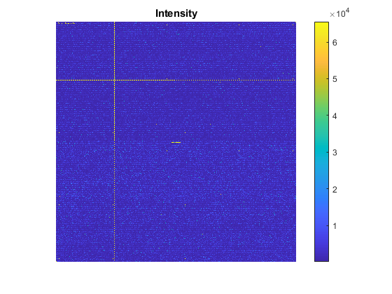
The affysnpquartets function creates a table of probe quartets for a SNP. On Affymetrix 100K SNP arrays, a probe quartet contains 20 probe pairs. For example, to get detailed information on probe set number 6540, you can type the following commands:

ps_id = 6540;
ps_qt = affysnpquartets(s_cel, s_cdf, ps_id)

ps_qt = 

  struct with fields:

    ProbeSet: '2685329'
     AlleleA: 'A'
     AlleleB: 'G'
     Quartet: [1×6 struct]

You can also view the heat map of the intensities of the PM and MM probe pairs of a SNP probe quartet using the probesetplot function. Click the Insert Colorbar button to show the color scale of the heat map.

probesetplot(s_cel, s_cdf, ps_id, 'imageonly', true);

In this view, the 20 probe pairs are ordered from left to right. The first two rows (10 probe pairs) correspond to allele A, and the last two rows (10 probe pairs) corresponds to allele B. For each allele, the left 5 probe pairs correspond to the sense strand (-), while the right 5 probe pairs correspond to the antisense (+) strand.

Importing and Converting the Data Set

You will use the celintensityread function to read all 24 CEL files. The celintensityread function returns a structure containing the matrices of PM and MM (optional) intensities for the probes and their group numbers. In each probe intensity matrix, the column indices correspond to the order in which the CEL files were read, and each row corresponds to a probe. For copy number (CN) analysis, only PM intensities are needed.

Import the probe intensity data of all EA 50KXba arrays into a MATLAB structure.

XbaData = celintensityread(cels, 'CentXbaAv2.cdf',...
                     'celpath', Xba_celPath, 'cdfpath', libPath)

Reading CDF file: CentXbaAv2.cdf
Reading file 1 of 24: H524
Reading file 2 of 24: H526
Reading file 3 of 24: H1184
Reading file 4 of 24: H1607
Reading file 5 of 24: H1963
Reading file 6 of 24: S0168T
Reading file 7 of 24: S0169T
Reading file 8 of 24: S0170T
Reading file 9 of 24: S0171T
Reading file 10 of 24: S0172T
Reading file 11 of 24: S0173T
Reading file 12 of 24: S0177T
Reading file 13 of 24: S0185T
Reading file 14 of 24: S0187T
Reading file 15 of 24: S0188T
Reading file 16 of 24: S0189T
Reading file 17 of 24: S0190T
Reading file 18 of 24: S0191T
Reading file 19 of 24: S0192T
Reading file 20 of 24: S0193T
Reading file 21 of 24: S0194T
Reading file 22 of 24: S0196T
Reading file 23 of 24: S0198T
Reading file 24 of 24: S0199T

XbaData = 

  struct with fields:

          CDFName: 'CentXbaAv2.cdf'
         CELNames: {1×24 cell}
         NumChips: 24
     NumProbeSets: 63434
        NumProbes: 1268480
      ProbeSetIDs: {63434×1 cell}
     ProbeIndices: [1268480×1 uint8]
     GroupNumbers: [1268480×1 uint8]
    PMIntensities: [1268480×24 single]

Affymetrix Early Access arrays are the same as the current commercial Mapping 100K arrays with the exception of some the probes being masked out. The data obtained from Affymetrix EA 100K SNP arrays can be converted to Mapping 100K arrays by filtering out the rejected SNP probe IDs on Early Access array and converting the SNP IDs to Mapping 100K SNP IDs. The SNP IDs for EA 50KXba and 50KHind arrays and their corresponding SNP IDs on Mapping 50KXba and 50KHind arrays are provided in two MAT files shipped with the Bioinformatics Toolbox software, Mapping50K_Xba_V_EA and Mapping50K_Hind_V_EA, respectively.

load Mapping50K_Xba_V_EA

The helper function affysnpemconvert converts the data to Mapping 50KXba data.

XbaData = affysnpemconvert(XbaData, EA50K_Xba_SNPID, Mapping50K_Xba_SNPID)

XbaData = 

  struct with fields:

          CDFName: 'CentXbaAv2.cdf'
         CELNames: {1×24 cell}
         NumChips: 24
     NumProbeSets: 58960
        NumProbes: 1179200
      ProbeSetIDs: {58960×1 cell}
     ProbeIndices: [1179200×1 uint8]
     GroupNumbers: [1179200×1 uint8]
    PMIntensities: [1179200×24 single]

Probe Intensity Normalization

You can view the density plots of the log-transformed PM intensity distribution across the 24 samples before preprocessing.

f=zeros(nSample, 100);
xi = zeros(nSample, 100);
for i = 1:nSample
   [f(i,:),xi(i,:)] = ksdensity(log2(XbaData.PMIntensities(:,i)));
end

figure;
plot(xi', f')
xlabel('log2(PM)')
ylabel('Density')
title('Density Plot')
hold on

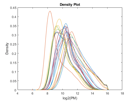
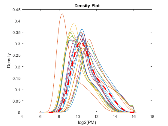
Quantile normalization is particularly effective in normalizing non-linearities in data introduced by experimental biases. Perform quantile normalization using the quantilenorm function.

XbaData.PMIntensities = quantilenorm(XbaData.PMIntensities);

Plot the resulting quantile distribution using a dashed red curve.

[f,xi] = ksdensity(log2(XbaData.PMIntensities(:,1)));
plot(xi', f', '--r', 'Linewidth', 3)
hold off

Note: You can also use the RMA or GCRMA procedures for background correction. The RMA procedure estimates the background by a mixture model where the background signals are assumed to be normally distributed and the true signals are exponentially distributed, while the GCRMA process consists of optical background correction and probe-sequence based background adjustment. For more information on how to use the RMA and GCRMA procedures, see Preprocessing Affymetrix Microarray Data at the Probe Level.

Probe-Level Summarization

By using the GroupNumbers field data from the structure XbaData, you can extract the intensities for allele A and allele B for each probe. Use the function affysnpintensitysplit to split the probe intensities matrix PMIntensities into two single-precision matrices, PMAIntensities and PMBIntensities, for allele A and allele B probes respectively. The number of probes in each matrix is the maximum number of probes for each allele.

XbaData = affysnpintensitysplit(XbaData)

XbaData = 

  struct with fields:

           CDFName: 'CentXbaAv2.cdf'
          CELNames: {1×24 cell}
          NumChips: 24
      NumProbeSets: 58960
         NumProbes: 589600
       ProbeSetIDs: {58960×1 cell}
      ProbeIndices: [589600×1 uint8]
    PMAIntensities: [589600×24 single]
    PMBIntensities: [589600×24 single]

For total copy number analysis, a simplification is to ignore the allele A and allele B sequences and their strand information and, instead, combine the PM intensities for allele A and allele B of each probe pair.

PM_Xba = XbaData.PMAIntensities + XbaData.PMBIntensities;

For a particular SNP, we now have K (K=5 for Affymetrix Mapping 100K arrays) added signals, each signal being a measure of the same thing - the total CN. However, each of the K signals has slightly different sequences, so their hybridization efficiency might differ. You can use RMA summarization methods to sum up allele probe intensities for each SNP probe set.

PM_Xba = rmasummary(XbaData.ProbeIndices, PM_Xba);

Getting SNP Probe Information

Affymetrix provides CSV-formatted annotation files for their SNP arrays. You can download the annotation files for Mapping 100K arrays from https://www.thermofisher.com/us/en/home/life-science/microarray-analysis/microarray-data-analysis/genechip-array-annotation-files.html.

For this example, download and unzip the annotation file for the Mapping, 50KXba array Mapping50K_Xba240.na29.annot.csv. The SNP probe information of the Mapping 50KXba array, can be read from this annotation file. Set the variable annoPath with the path to the location where you saved the annotation file.

annoPath = 'C:\Examples\affysnpcnvdemo\AnnotFiles';

The function affysnpannotread reads the annotation file and returns a structure containing SNP chromosome information, chromosomal positions, sequences and PCR fragment length information ordered by probe set IDs from the second input variable.

annoFile = fullfile(annoPath, 'Mapping50K_Xba240.na29.annot.csv');
annot_Xba = affysnpannotread(annoFile, XbaData.ProbeSetIDs)

annot_Xba = 

  struct with fields:

       ProbeSetIDs: {58960×1 cell}
        Chromosome: [58960×1 int8]
     ChromPosition: [58960×1 double]
          Cytoband: {58960×1 cell}
          Sequence: {58960×1 cell}
           AlleleA: {58960×1 cell}
           AlleleB: {58960×1 cell}
         Accession: {58960×1 cell}
    FragmentLength: [58960×1 double]

Raw CN Estimation

The relative copy number at a SNP between two samples is estimated based on the log2 ratio of the normalized signals. The averaged normalized signals from normal samples are used as the global reference. The preprocessed reference mean log-transformed signals for the Mapping 50KXBa array and the 50KHind array are provided in the MAT-files, SCLC_normal_Xba and SCLC_normal_Hind respectively.

load SCLC_Normal_Xba

Estimate the log2 ratio of normalized signals.

log2Ratio_Xba = bsxfun(@minus, PM_Xba, mean_normal_PM_Xba);

Filtering and Ordering

SNPs probes with missing chromosome number, genomic position or fragment length in the annotation file don't have enough information for further CN analysis. Also for CN analysis, Y chromosomes are usually ignored. Filter out these SNP probes.

fidx = annot_Xba.Chromosome == -1 | annot_Xba.Chromosome == 24 |...
       annot_Xba.ChromPosition == -1 | annot_Xba.FragmentLength == 0;
log2Ratio_Xba(fidx, :) = [];
chromosome_Xba = annot_Xba.Chromosome(~fidx);
genomepos_Xba = annot_Xba.ChromPosition(~fidx);
probesetids_Xba = XbaData.ProbeSetIDs(~fidx);
fragmentlen_Xba = annot_Xba.FragmentLength(~fidx);
accession_Xba = annot_Xba.Accession(~fidx);

Order CN estimation by chromosomes numbers:

[chr_sort, sidx] = sort(chromosome_Xba);
gpos_sort = genomepos_Xba(sidx);
log2Ratio_sort = log2Ratio_Xba(sidx, :);
probesetids_sort = probesetids_Xba(sidx);
fragmentlen_sort = fragmentlen_Xba(sidx);
accession_sort = accession_Xba(sidx);

Order CN estimation by chromosomal genomic positions:

u_chr = unique(chr_sort);
gpsidx = zeros(length(gpos_sort),1);
for i = 1:length(u_chr)
    uidx = find(chr_sort == u_chr(i));
    gp_s = gpos_sort(uidx);
    [gp_ss, ssidx] = sort(gp_s);
    s_res = uidx(ssidx);
    gpsidx(uidx) = s_res;
end

gpos_ssort = gpos_sort(gpsidx);
log2Ratio_ssort = log2Ratio_sort(gpsidx, :);
probesetids_ssort = probesetids_sort(gpsidx);
fragmentlen_ssort = fragmentlen_sort(gpsidx);
accession_ssort = accession_sort(gpsidx);

PCR Fragment Length Normalization

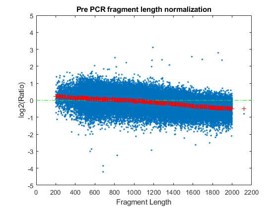
In the analysis, systematic effects from the PCR process should be taken into account. For example, longer fragments usually result in less PCR amplification, which leads to less material to hybridize and weaker signals. You can see this by plotting the raw CNs with fragment-length effect.

figure;
plot(fragmentlen_ssort, log2Ratio_ssort(:, 1), '.')
hold on
plot([0 2200], [0 0], '-.g')
xlim([0 2200])
ylim([-5 5])
xlabel('Fragment Length')
ylabel('log2(Ratio)')
title('Pre PCR fragment length normalization')

Nannya et al., 2005 introduced a robust linear model to estimate and remove this effect. For this example, use the malowess function for PCR fragment length normalization for sample 1. Then display the smooth fit curve.

smoothfit = malowess(fragmentlen_ssort,log2Ratio_ssort(:,1));
hold on
plot(fragmentlen_ssort, smoothfit, 'r+')
hold off

log2Ratio_norm = log2Ratio_ssort(:,1) - smoothfit;

Plot the PCR fragment length normalized raw CN estimation:

figure;
plot(fragmentlen_ssort, log2Ratio_norm, '.');
hold on
plot([0 2200], [0 0], '-.g')
xlim([0 2200])
ylim([-5 5])
xlabel('Fragment Length')
ylabel('log2(Ratio)')
title('Post PCR fragment length normalization')
hold off

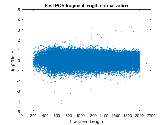
You can normalize PCR fragment length effect for all the samples using the malowess function.

Again, you can repeat the previous steps for the 50KHind array data.

CN Genome Profile

Load a MAT-file containing the preprocessed and normalized CN data from both the 50KXba arrays and 50KHind arrays.

load SCLC_CN_Data

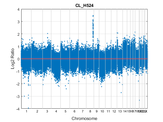
You can now plot the whole-genome profile of total CNs. For example, plot the whole-genome profile for sample 1 (CL_H524) using a helper function plotcngenomeprofile.

plotcngenomeprofile(SCLC_CN.GenomicPosition,SCLC_CN.Log2Ratio(:, 1),...
                  SCLC_CN.Chromosome, 1:23, SCLC_CN.Sample{1})

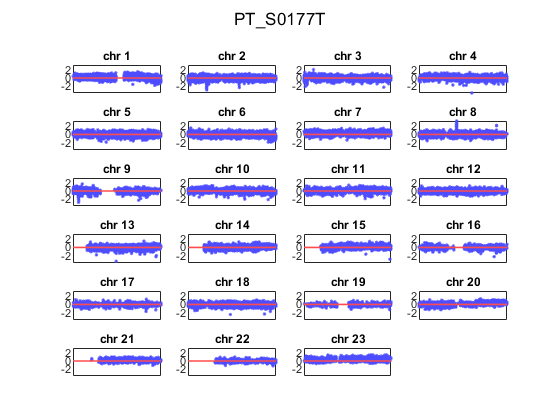
You can also plot each chromosome CN profile in a subplot. For example, plot each chromosome CN profile for sample 12 (PT_0177T):

plotcngenomeprofile(SCLC_CN.GenomicPosition,SCLC_CN.Log2Ratio(:, 12),...
                  SCLC_CN.Chromosome, 1:23, SCLC_CN.Sample{12}, 'S')

8q Amplification in SCLS Samples

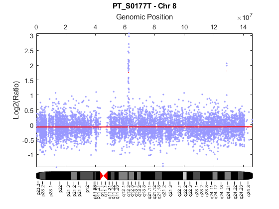
In the Zhao et al., 2005 study, a high-level amplification was observed in the q12.2-q12.3 region on chromosome 8 for SCLS samples. You can perform CBS segmentation on chromosome 8 for sample PT_S0177T.

sampleid = find(strcmpi(samples, 'PT_S0177T'));
ps = cghcbs(SCLC_CN, 'sampleind', sampleid, 'chromosome', 8, 'showplot', 8)

Analyzing: PT_S0177T. Current chromosome 8

ps = 

  struct with fields:

         Sample: 'PT_S0177T'
    SegmentData: [1×1 struct]

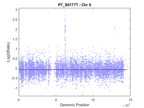
Add the ideogram for chromosome 8 to the plot:

chromosomeplot('hs_cytoBand.txt', 8, 'addtoplot', gca)

Infer copy number changes:

segment_cn = ceil((2.^ps.SegmentData.Mean)*2);
cnv = segment_cn(segment_cn ~= 2);
startbp = ps.SegmentData.Start(segment_cn ~= 2)
endbp = ps.SegmentData.End(segment_cn ~= 2)
startMB = startbp/10^6;
endMB = endbp/10^6;

You can also get cytoband information for the CNVs. The function cytobandread returns cytoband information in a structure.

ct = cytobandread('hs_cytoBand.txt')

ct = 

  struct with fields:

     ChromLabels: {862×1 cell}
    BandStartBPs: [862×1 int32]
      BandEndBPs: [862×1 int32]
      BandLabels: {862×1 cell}
       GieStains: {862×1 cell}

Find cytoband labels for CNVs:

cn_cytobands = cell(length(cnv),1);
for i = 1:length(cnv)
    istart = find(ct.BandStartBPs <= startbp(i) & ct.BandEndBPs >= startbp(i) & strcmp(ct.ChromLabels, '8'));
    iend = find(ct.BandStartBPs <= endbp(i) & ct.BandEndBPs >= endbp(i) & strcmpi(ct.ChromLabels, '8'));
    if strcmpi(ct.BandLabels{istart}, ct.BandLabels{iend})
        cn_cytobands{i} = ['8' ct.BandLabels{istart}];
    else
        cn_cytobands{i} = ['8' ct.BandLabels{istart} '-' '8' ct.BandLabels{iend}];
    end
end

Create a report displaying the start positions, end positions and size of the CNVs.

report = sprintf('Cytobands      \tStart(Mb)\tEnd(Mb)\t\tSize(Mb)\tCN\n');
for i = 1:length(cnv)
   report = sprintf('%s%-15s\t%3.2f\t\t%3.2f\t\t%3.2f\t\t%d\n',...
               report, cn_cytobands{i},startMB(i),endMB(i),endMB(i)-startMB(i),cnv(i));
end
disp(report)

Cytobands      	Start(Mb)	End(Mb)		Size(Mb)	CN
8q12.2         	62.09		62.18		0.09		4
8q12.2-8q12.3  	62.18		62.73		0.55		7
8q24.21        	128.77		129.01		0.24		7

Among the three regions of amplification, the 8q12-13 region has been confirmed by interphase FISH analysis (Zhao et al., 2005).

CN Gain/Loss Summary Plot

You can also visualize the fraction of samples with copy number amplifications of at least three copies (red), and copy number losses to less than 1.5 copies (blue), across all SNPs for all SCLS samples. The function cghfreqplot displays frequency of copy number alterations across multiple samples. To better visualize the data, plot only the SNPs with gain or loss frequency over 25%.

gainThrd = log2(3/2);
lossThrd = log2(1.5/2);
cghfreqplot(SCLC_CN, 'Color', [1 0 0; 0 0 1],...
            'Threshold', [gainThrd, lossThrd], 'cutoff', 0.25)
title('SCLC Summary Plot')

References

[1] Zhao, X., et al., "Homozygous deletions and chromosome amplifications in human lung carcinomas revealed by single nucleotide polymorphism array analysis", Cancer Research, 65(13):5561-70, 2005.

[2] Nannya, Y., et al., "A robust algorithm for copy number detection using high-density oligonucleotide single nucleotide polymorphism genotyping arrays", Cancer Research, 65(14):6071-8, 2005.