Generate Code for Segmentation Application Using Quantized LiteRT Model (Tech Preview)

R2026b

Since R2026b

This example shows how to generate CUDA code for quantized LiteRT models. For more information, see Code Generation for Quantized LiteRT Models (Tech Preview).

Note

Code generation for quantized LiteRT models is a tech preview feature. This feature is in active development and might change between the tech preview and the general release. The primary purpose of the tech preview is to solicit feedback from users. To enable this feature, enter enableCodegenForQuantizedLiteRTModels at the command line before calling the loadLiteRTModel function or loading a model by using the LiteRT block. To provide feedback, email the development team or participate in a survey.

Generate Code for Quantized LiteRT Models Using YOLO v11 Segmentation

This example shows how to generate CUDA® code for quantized int8 LiteRT models and compare their deployment size and inference performance against a float32 baseline. The example uses a YOLO v11 instance segmentation model trained by Ultralytics on the COCO data set. You generate code for three model variants (float32, dynamic int8 quantization, and full integer int8 quantization), and compare their segmentation results, deployment artifact size, and inference latency. The generated CUDA code does not depend on any third-party deep learning libraries.

Third-Party Prerequisites

This example requires a CUDA-enabled NVIDIA® GPU and a compatible driver.

For non-MEX builds, such as static, dynamic libraries or executables, this example also requires:

• The NVIDIA CUDA toolkit.

• Environment variables for the compilers and libraries. For more information, see Third-Party Hardware (GPU Coder) and Setting Up the Prerequisite Products (GPU Coder).

Verify GPU Environment

To verify that the compilers and libraries for this example are set up correctly, use the coder.checkGpuInstall (GPU Coder) function.

envCfg = coder.gpuEnvConfig("host");
envCfg.DeepCodegen = 1;
envCfg.Quiet = 1;
coder.checkGpuInstall(envCfg);

Download Pretrained Models

This example uses pretrained YOLO v11 instance segmentation models trained on the COCO data set. The models can detect and identify 80 different objects. Use this code to download the YOLO v11 models in LiteRT format from the YOLO v11 GitHub repository.

baseUrl = ["https://raw.githubusercontent.com/" ...
    "matlab-deep-learning/" ...
    "pretrained-yolo-v11-litert-model-for-segmentation-and-object-detection-with-matlab/" ...
    "main/"];

modelFiles = {"yolo11s-seg_float32.tflite", ...
    "yolo11s-seg_int8_dynamic_quant.tflite", ...
    "yolo11s-seg_integer_quant.tflite"};

for i = 1:numel(modelFiles)
    if ~isfile(modelFiles{i})
        fprintf("Downloading %s...\n", modelFiles{i});
        websave(modelFiles{i}, strjoin([baseUrl modelFiles{i}],""));
    end
end

Downloading yolo11s-seg_float32.tflite...
Downloading yolo11s-seg_int8_dynamic_quant.tflite...
Downloading yolo11s-seg_integer_quant.tflite...

This example compares three model variants that differ in how weights and computations are represented:

• float32 baseline — all weights and activations use 32-bit floating point. This is the standard, unquantized model.

• Dynamic int8 quantization — weights are stored as int8 (~4x smaller model file), but are dequantized back to float32 at runtime. All computation is performed in float32. You do not need to calibrate data when you export the model.

• Integer int8 quantization — both weights and activations are quantized to int8, and arithmetic is performed in int8 internally. float32 is used only at the model I/O boundary. This requires calibration data during export but can yield better performance on hardware with native int8 compute units.

Examine the yoloSegmentImageQuant Entry-Point Function

The yoloSegmentImageQuant entry-point function takes an input image, a model file path, and an output order vector. It loads the specified LiteRT model using loadLiteRTModel, runs inference with invoke, and postprocesses the outputs into annotated bounding boxes and segmentation masks. Use the outputOrder argument to specify the order of detection and mask outputs, which can differ between model variants.

type("yoloSegmentImageQuant.m")

function out = yoloSegmentImageQuant(in, modelPath, outputOrder)
% Copyright 2026 The MathWorks, Inc.
%#codegen
coder.gpu.kernelfun;

origSize = size(in, 1:2);
inputSize = [640 640];
img = im2single(imresize(in, inputSize));

persistent yoloSegModel

if isempty(yoloSegModel)
    yoloSegModel = loadLiteRTModel(modelPath);
end

outs = cell(1, 2);
[outs{:}] = invoke(yoloSegModel,permute(img, [4 1 2 3]));
outputs = permute(outs{outputOrder(1)}, [3 2 1]);
masks = squeeze(outs{outputOrder(2)});

bboxIndices = 1:4;
scoresIndices = 5:84;

allBboxes = outputs(:, bboxIndices);
[allScores, allLabels] = max(outputs(:, scoresIndices), [], 2);
keep = allScores > 0.5;

bboxes = allBboxes(keep, :);
bboxes(:, [1 3]) = bboxes(:, [1 3]) * origSize(2);
bboxes(:, [2 4]) = bboxes(:, [2 4]) * origSize(1);

% boxes are in [xctr, yctr, w, h] form -> convert to format expected by NMS
% in MATLAB
bboxes = convertCenterBboxesToTopLeft(bboxes);
scores = allScores(keep);
labels = allLabels(keep);

[bboxesNMS, ~, labelsNMS, nmsIndices] = selectStrongestBboxMulticlass(bboxes, scores, labels,...
    'RatioType', 'Min', 'OverlapThreshold', 0.8);

classes = createCOCOClasses(labelsNMS);

maskCoeffs = outputs(keep, scoresIndices(end)+1:end);
maskCoeffs = maskCoeffs(nmsIndices, :);
binaryMasks = processMasks(masks, maskCoeffs, topLeftBboxToXYXY(bboxesNMS), origSize);
RGB = insertObjectMask(in,binaryMasks,LineColor=[1 1 1],LineWidth=1);
out = insertObjectAnnotation(RGB, 'rectangle', bboxesNMS, classes);

end

Display the Test Image

Load the test image for segmentation and object detection.

I = imread("downtownScene.jpg");
imshow(I);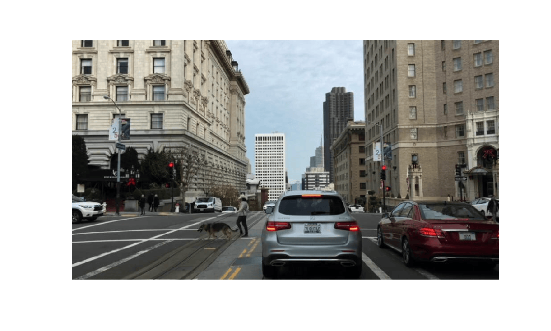

Generate and Execute float32 Model

Generate CUDA code for the float32 baseline model. Use the coder.gpuConfig function to create a MEX code configuration object and run the codegen command. The model path and output order are passed as compile-time constants by using coder.Constant(), allowing the same entry-point to be reused across the float32 and quantized model variants. For the float32 model, detections are the first output and masks are the second, so the output order is [1 2].

float32Model = fullfile(pwd, "yolo11s-seg_float32.tflite");
detFirst = [1 2];
cfg = coder.gpuConfig;
codegen -config cfg yoloSegmentImageQuant -args {I, coder.Constant(float32Model), coder.Constant(detFirst)} -o yoloSegFloat32_mex -d codegen/float32

Code generation successful: View report

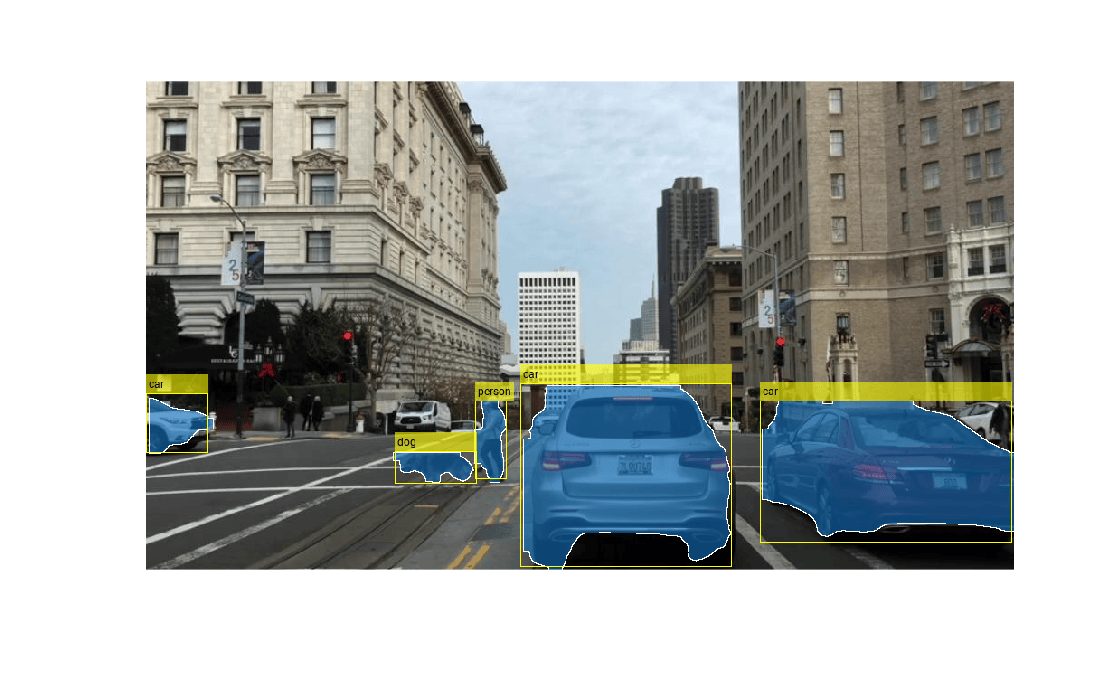
Visualize the segmented image by running the generated executable.

out = yoloSegFloat32_mex(I, float32Model, detFirst);
imshow(out);

Enable Tech Preview Feature for Quantized Models

Code generation for quantized LiteRT models is a tech preview feature. You must explicitly enable it before use. Attempting to generate code for a quantized model without enabling the feature produces an error. For more information, see Code Generation for Quantized LiteRT Models (Tech Preview).

Enable code generation for quantized LiteRT models.

enableCodegenForQuantizedLiteRTModels();

=== Code generation for quantized LiteRT models is ENABLED ===

For feature overview, see Code Generation for Quantized LiteRT Models (Tech Preview). To send feedback or questions directly to the development team, email [e-mail] or click here to take survey.

Generate and Execute Dynamic int8 Quantized Model

Generate CUDA code for the dynamically quantized model. This model stores weights as int8 but dequantizes them to float32 at runtime. The quantized models maintain the same float32 input/output interface as the baseline, so the entry-point function remains unchanged.

dynamicQuantModel = fullfile(pwd,"yolo11s-seg_int8_dynamic_quant.tflite");
cfg = coder.gpuConfig;
codegen -config cfg yoloSegmentImageQuant -args {I, coder.Constant(dynamicQuantModel), coder.Constant(detFirst)} -o yoloSegDynQuant_mex -d codegen/dynQuant

Code generation successful: View report

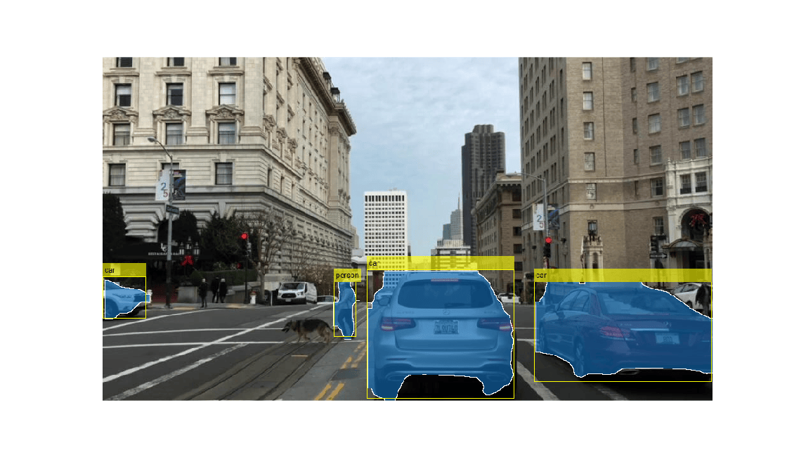
Run the dynamic int8 quantized model on the image and visualize the segmentation result. The outputs might differ slightly from the float32 baseline because of quantization loss — small numeric differences in confidence scores and bounding box coordinates can cause minor variations in which detections pass the confidence threshold or survive non-maximum suppression (NMS).

outDynQuant = yoloSegDynQuant_mex(I, dynamicQuantModel, detFirst);
imshow(outDynQuant);

Generate and Execute Integer int8 Quantized Model

Generate CUDA code for the integer quantized model. This model performs arithmetic in int8 internally, using float32 only at the I/O boundary. The integer quantized model returns outputs in a different order, so the output order is set to [2 1].

integerQuantModel = fullfile(pwd, "yolo11s-seg_integer_quant.tflite");
detSecond = [2 1];
cfg = coder.gpuConfig;
codegen -config cfg yoloSegmentImageQuant -args {I, coder.Constant(integerQuantModel), coder.Constant(detSecond)} -o yoloSegIntQuant_mex -d codegen/intQuant

Code generation successful: View report

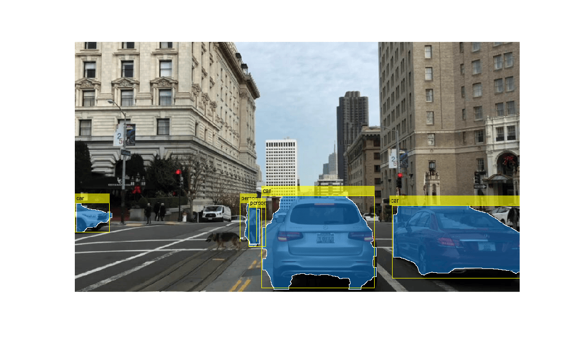
Run the integer int8 quantized model on the image and visualize the segmentation result. Visualize the segmented image produced by the integer quantized model. Similar to dynamic int8 quantization, the integer int8 quantized model outputs might differ slightly from the float32 baseline due to reduced precision.

outIntQuant = yoloSegIntQuant_mex(I, integerQuantModel, detSecond);
imshow(outIntQuant);

Deployment Size and Performance Comparison

Call the helper function compareDeploymentMetrics to compare the deployment artifact size and inference time across all three variants.

compareDeploymentMetrics(I, ...
    {@yoloSegFloat32_mex, @yoloSegDynQuant_mex, @yoloSegIntQuant_mex}, ...
    {float32Model, dynamicQuantModel, integerQuantModel}, ...
    {detFirst, detFirst, detSecond}, ...
    {fullfile(pwd,"codegen","float32"), fullfile(pwd,"codegen","dynQuant"), fullfile(pwd,"codegen","intQuant")}, ...
    {"yoloSegFloat32_mex.mexa64", "yoloSegDynQuant_mex.mexa64", "yoloSegIntQuant_mex.mexa64"}, ...
    {"Float32", "Int8 (dynamic)", "Int8 (integer)"});

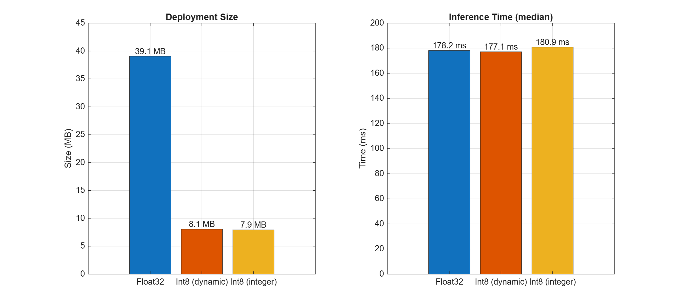
The quantized models are approximately four times smaller than the float32 baseline. The dynamic quantized model has inferernce time similar to the float32 baseline because the model still uses float32 at runtime. The integer quantized model performs int8 arithmetic internally.

Helper Function

The compareDeploymentMetrics function benchmarks and visualizes deployment size and inference time for multiple generated MEX variants.

Inputs:

• I — Test image passed to each MEX function.

• mexFcns — Cell array of function handles to the generated MEX functions (for example, {@myMex_float32, @myMex_int8}).

• modelPaths — Cell array of full paths to the model files.

• outputOrders — Cell array of output order vectors for each variant.

• codegenDirs — Cell array of code generation output directories containing the MEX and .bin files.

• mexNames — Cell array of MEX file names (for example, {"myMex_float32.mexa64", "myMex_int8.mexa64"}).

• variantLabels — Cell array of display labels for the bar chart x-axis.

function compareDeploymentMetrics(I, mexFcns, modelPaths, outputOrders, codegenDirs, mexNames, variantLabels)
% Compare deployment size and inference time across model variants.

nVariants = numel(mexFcns);
nRuns = 20;
times = zeros(nVariants, nRuns);

% Warm-up
for v = 1:nVariants
    feval(mexFcns{v}, I, modelPaths{v}, outputOrders{v});
end

% Benchmark
for i = 1:nRuns
    for v = 1:nVariants
        tic;
        feval(mexFcns{v}, I, modelPaths{v}, outputOrders{v});
        times(v, i) = toc;
    end
end

% Compute deployment sizes (MEX + .bin files)
sizes = zeros(1, nVariants);
for v = 1:nVariants
    binFiles = dir(fullfile(codegenDirs{v}, "*.bin"));
    mexFile = dir(fullfile(codegenDirs{v}, mexNames{v}));
    sizes(v) = sum([binFiles.bytes]) + sum([mexFile.bytes]);
end
sizes = sizes / 1e6;
medianTimes = median(times, 2)' * 1000;

% Use a consistent color per variant across both plots
variantColors = lines(nVariants);

% Plot deployment size
figure("Position", [100 100 1100 500]);
subplot(1,2,1);
bSize = bar(sizes, "FaceColor", "flat");
bSize.CData = variantColors;
set(gca, "XTickLabel", variantLabels);
ylabel("Size (MB)");
title("Deployment Size");
grid on;
for k = 1:nVariants
    text(k, sizes(k), sprintf("%.1f MB", sizes(k)), ...
        "HorizontalAlignment", "center", "VerticalAlignment", "bottom");
end
ylim([0 45]);

% Plot inference time
subplot(1,2,2);
bTime = bar(medianTimes, "FaceColor", "flat");
bTime.CData = variantColors;
set(gca, "XTickLabel", variantLabels);
ylabel("Time (ms)");
title("Inference Time (median)");
grid on;
for k = 1:nVariants
    text(k, medianTimes(k), sprintf("%.1f ms", medianTimes(k)), ...
        "HorizontalAlignment", "center", "VerticalAlignment", "bottom");
end
end

References

[1] Lin, Tsung-Yi, Michael Maire, Serge Belongie, et al. “Microsoft COCO: Common Objects in Context.” In Computer Vision – ECCV 2014, edited by David Fleet, Tomas Pajdla, Bernt Schiele, and Tinne Tuytelaars, vol. 8693. Springer International Publishing, 2014. https://doi.org/10.1007/978-3-319-10602-1_48.