Compare Robust Fitting Methods

This example shows how to fit a polynomial model to data using the bisquare weights, least absolute residuals (LAR), and linear least-squares methods.

Create a vector of noisy data by using the function randn.

rng("default")  % Set the seed for reproducibility
noise = randn([200,1]);

Create a vector of evenly spaced points between 0 and 2$\pi$ by using the linspace function. Create a vector of sample data by adding the noisy data to one sine wave cycle.

theta = linspace(0,2*pi,200)';
data = sin(theta) + noise;

Add outliers to the data by replacing every tenth value of data with a random value from the normal distribution. Specify a mean of 5 and standard deviation of 1 for the random values.

for i=10:10:200
    data(i) = randn+5;
end

Display a box plot of the sample data.

boxchart(data)

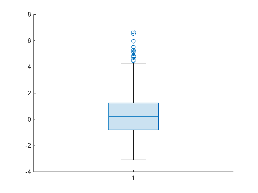
Place your cursor on the box plot to display the box plot statistics.

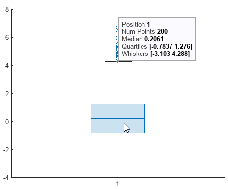
The figure indicates that the outliers are data points with values greater than 4.288.

Fit four third-degree polynomial models to the data by using the function fit with different fitting methods. Use the two robust least-squares fitting methods: bisquare weights method to calculate the coefficients of the first model, and the LAR method to calculate the coefficients of the third model. Use the linear least-squares method to calculate the coefficients of the second and fourth models. To remove the outliers from the data in the fitting of the fourth model, exclude data points greater than 4.288.

bisquarepolyfit = fit(theta,data,"poly3",'Robust',"Bisquare");
linearpolyfit = fit(theta,data,"poly3");
larpolyfit = fit(theta,data,"poly3",Robust="LAR");
excludeoutlierspolyfit = fit(theta,data,"poly3",...
    Exclude=data>4.288);

Compare the bisquare weights and linear least-squares fits by plotting them in the same plot with the data.

plot(bisquarepolyfit,theta,data)
hold on
plot(linearpolyfit,"g")
legend("data","bisquare weights fit","linear least-squares fit")
xlabel("theta")
ylabel("data")
hold off

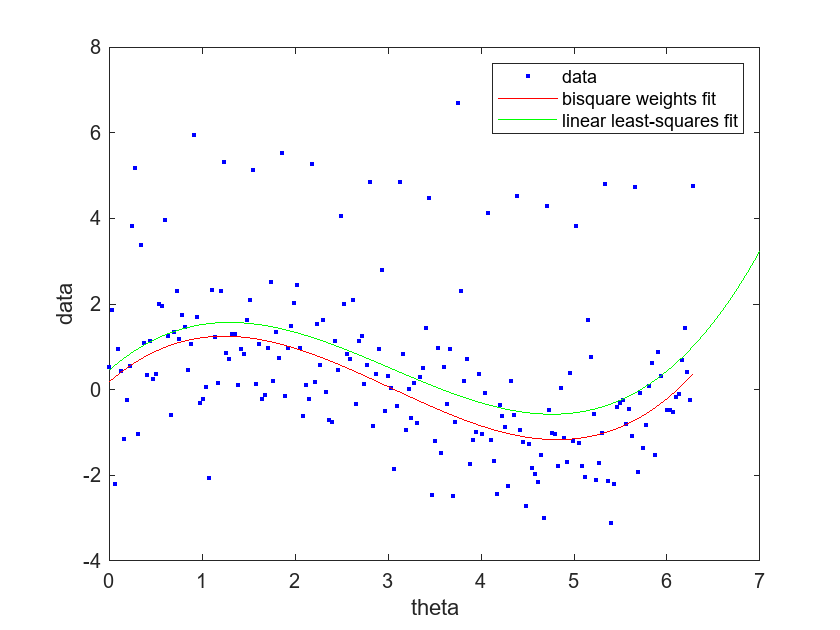
As shown in the plot, the curve of the linear-least squares fit is higher and closer to the outliers than the curve of the bisquare weights fit. The curve of the bisquare weights fit is more central to the bulk of the data. The relative positions of the curves indicate that the outliers have a larger effect on the linear least-squares fit.

Compare the bisquare weights and LAR fits.

plot(bisquarepolyfit,theta,data)
hold on
plot(larpolyfit,"g")
legend("data","bisquare weights fit","LAR fit")
xlabel("theta")
ylabel("data")
hold off

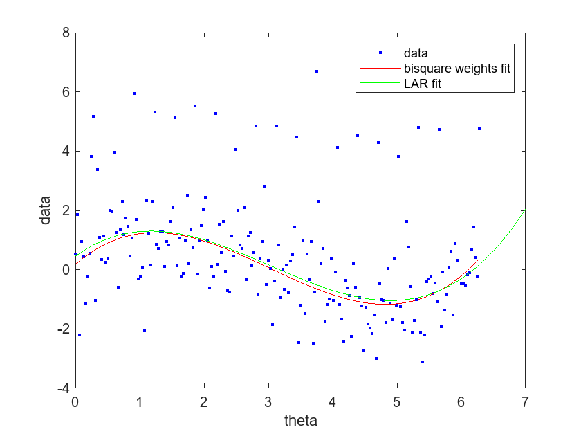
The curve of the LAR fit follows the curve of the bisquare weights fit closely, and is not as influenced by the outliers compared to the linear least-squares fit. You can zoom in to the plot to see that the curve of the LAR fit is slightly higher than the curve of the bisquare weights fit for most values of theta.

Compare the bisquare weights fit to the linear-least squares fit without outliers.

plot(bisquarepolyfit,theta,data)
hold on
plot(excludeoutlierspolyfit,"g")
legend("data","bisquare weights fit","linear least-squares fit (without outliers)")
xlabel("theta")
ylabel("data")
hold off

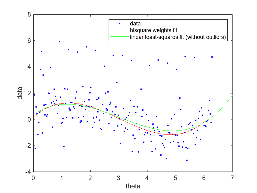
The linear-least squares fit does not appear to be greatly influenced by the outliers. However, the fit is not as central to the bulk of the data compared to the bisquare weights fit. Together, the plots indicate that, out of the four models, the model fit with the bisquare weights method is the most central to the bulk of the data.