csaps
Cubic smoothing spline
Syntax
Description
Note
For a simpler but less flexible method to generate smoothing splines, try the Curve Fitter
app or the fit function.
pp = csaps(x,y)(x,y)
in ppform. The value of spline f at data site x(j)
approximates the data value y(:,j) for j =
1:length(x).
The smoothing spline f minimizes
Here, n is the number of entries of x and the
integral is over the smallest interval containing all the entries of x.
yj and
xj refer to the
jth entries of y and x,
respectively. D2f denotes
the second derivative of the function f.
The default values for the error measure weights
wj are 1. The default value
for the piecewise constant weight function λ in the roughness measure is the constant function 1. By default,
csaps chooses a value for the smoothing parameter p based on the given data sites
x.
To evaluate a smoothing spline outside its basic interval, you must first extrapolate
it. Use the command pp = fnxtr(pp) to ensure that the second derivative
is zero outside the interval spanned by the data sites.
[___] = csaps({x1,...,xm},
provides the ppform of an y,___)m-variate tensor-product smoothing spline to
data on the rectangular grid described by {x1,...,xm}. You can use this
syntax with any of the arguments in the previous syntaxes.
Examples
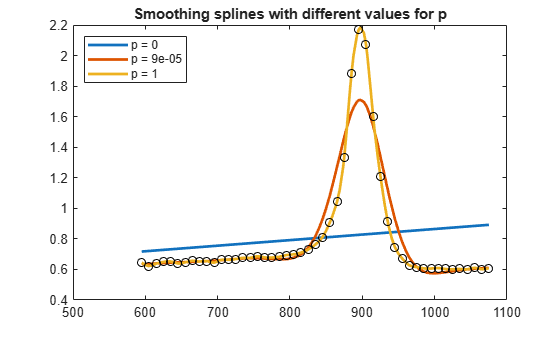
Fit smoothing splines using the csaps function with different values for the smoothing parameter p. Use values of p between the extremes of 0 and 1 to see how they affect the shape and closeness of the fitted spline.
Load the titanium data set.
[x, y] = titanium();
When p = 0, s0 is the least-squares straight line fit to the data. When p = 1, s1 is the variational, or natural, cubic spline interpolant.
For 0 < p < 1, sp is a smoothing spline that is a trade-off between the two extremes: smoother than the interpolant s1 and closer to the data than the straight line s0.
p = 0.00009;

s0 = csaps(x,y,0);
sp = csaps(x,y,p);
s1 = csaps(x,y,1);
figure
fnplt(s0);
hold on
fnplt(sp);
fnplt(s1);
plot(x,y,'ko');
hold off
title('Smoothing splines with different values for p');
legend('p = 0', ['p = ' num2str( p )], 'p = 1', 'Location', 'northwest')
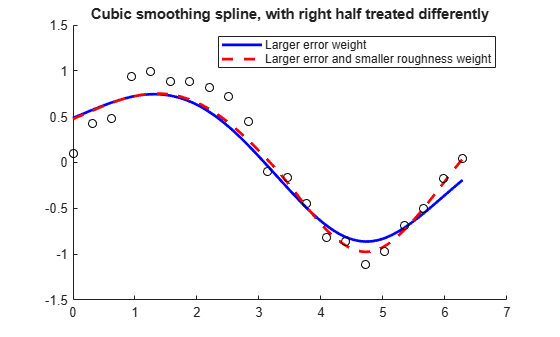
Adjust the smoothing parameter, error measure weights, and roughness measure weights.
Create a sine curve with noise.
x = linspace(0,2*pi,21); y = sin(x)+(rand(1,21)-.5)*.3;
Fit a smoothing spline to the data. Specify the smoothing parameter p = 0.4 and error measure weights w that vary across the data.
pp = csaps(x,y,0.4,[],[ones(1,10),repmat(5,1,10), 0]);
The function returns a smooth fit to the noisy data that is much closer to the data in the right half because of the much larger error measure weight there. Note that the error weighting of zero for the last data point excludes this point from the fit.
Now fit a smoothing spline using the same data, smoothing parameter and error measure weights, but with adjusted roughness measure weights.
pp1 = csaps(x,y, [.4,ones(1,10),repmat(.2,1,10)], [], ...
                    [ones(1,10), repmat(5,1,10), 0]);
The roughness measure weight is only 0.2 in the right half of the interval. Correspondingly, the fit is rougher but closer on the right side of the data (except for the last data point, which is ignored).
Plot both fits for comparison.
figure
hold on
fnplt(pp, 'b');
fnplt(pp1,'r--')
plot(x,y,'ok')
hold off
ylim([-1.5 1.5])
title(['Cubic smoothing spline, with right half treated ',...
          'differently'])
legend('Larger error weight', 'Larger error and smaller roughness weight')
Fit a smoothing spline to bivariate data generated by the peaks function with added uniform noise. Use csaps to obtain the new, smoothed data points and the smoothing parameters csaps determines for the fit.
Create the grid. For this example, the grid is a 51-by-61 uniform grid.
x = {linspace(-2,3,51),linspace(-3,3,61)};
[xx,yy] = ndgrid(x{1},x{2});
Generate the noisy data using the peaks function and random numbers in the interval .
y = peaks(xx, yy);
noisy = y + (rand(size(y)) - 0.5);
figure
surf(xx,yy,noisy)
axis off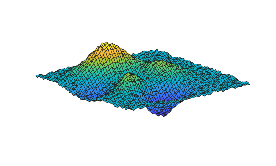
Fit the data. Use csaps to obtain the smoothed data values evaluated over the grid x and the default smoothing parameter used in the fit.
[sval,p] = csaps(x,noisy,[],x);
The plot of the fit shows that some roughness remains. Note that you must transpose the array sval.
figure
surf(x{1},x{2},sval.')
axis off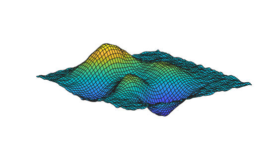
For a somewhat smoother approximation, specify a value for p that is slightly smaller than the csaps default value.
ssval = csaps(x,noisy,.996,x);
figure
surf(x{1},x{2},ssval.')
axis off
Input Arguments
Output Arguments
Algorithms
csaps is an implementation of the Fortran routine
SMOOTH from PGS.
The calculation of the smoothing spline requires solving a linear system whose coefficient
matrix has the form p*A + (1-p)*B, with the matrices A
and B depending on the data sites x. The default value
of p makes p*trace(A) equal
(1-p)*trace(B).
Version History
Introduced before R2006a