Solve PDE Using Fourier Neural Operator

R2026b

This example shows how to train a Fourier neural operator (FNO) neural network that outputs the solution of a partial differential equation (PDE).

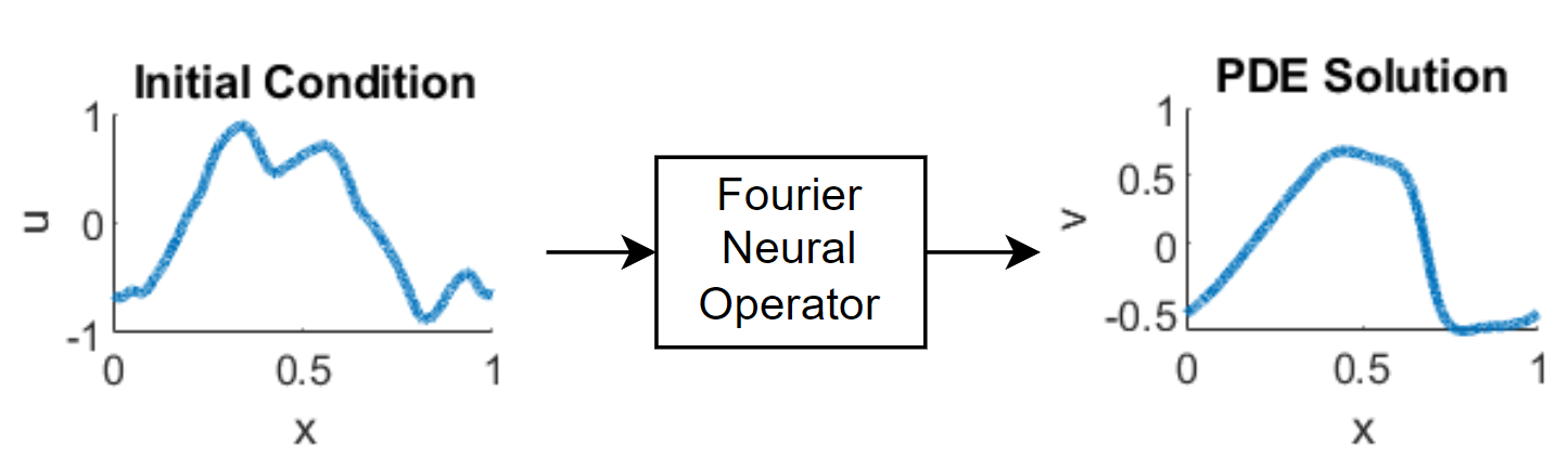
A neural operator [1] is a type of neural network that maps between function spaces. For example, it can learn to output the solution to a PDE when given the initial conditions for the system. A Fourier neural operator (FNO) [2] is a neural operator that can learn these mappings more efficiently by leveraging Fourier transforms. In particular, for an input function $f$ in the spatial domain, the layers in the neural network learn the transformation $F$ such that $F (f) = f_{}^{ˆ}$ , where $f_{}^{ˆ}$ is the Fourier transform of $f$ . The FNO can then operate in the frequency domain. Using a neural network to predict the solutions of a PDE can be faster than computing the solutions numerically.

This diagram illustrates the flow of data through an FNO.

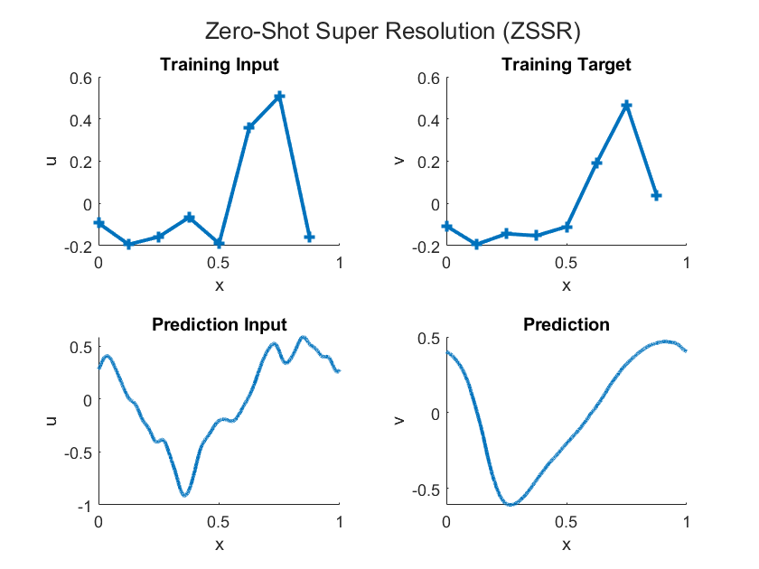
Diagram of data flowing through FNO. The input is a function labeled "Initial Condition". The output is a function labeled "PDE Solution".

Because an FNO learns mappings between function spaces, you can evaluate the output function at a higher resolution than that of the training data. This functionality is known as zero-shot super-resolution (ZSSR). That is, ZSSR is the ability to enhance the resolution of the input and output data beyond the original training data, without the need for additional high-resolution examples. This diagram illustrates the differences between low-resolution training data and high-resolution inputs and outputs for prediction.

Plots showing low resolution and high resolution inputs and outputs. The low-resolution functions are composed of a small number of straight lines between points. The high-resolution functions are smooth curves.

This example trains an FNO to output the solutions to the 1-D Burgers' equation.

Load Training Data

Load the data for the 1-D Burgers' equation.

The Burgers' equation is a PDE that arises in different areas of applied mathematics, for example, in fluid mechanics, nonlinear acoustics, gas dynamics, and traffic flows. The PDE is:

$\frac{\partial u}{\partial t} + u \frac{\partial u}{\partial x} = \frac{1}{R e} \frac{\partial^{2} u}{\partial x^{2}}, x \in (0, 1), t \in (0, 1),$

where $R e$ is the Reynolds number. The initial conditions are:

$u (x, 0) = u_{0} (x), x \in (0, 1)$

The equation imposes periodic boundary conditions across the spatial domain. The goal is to learn the mapping from the initial condition $u_{0}$ to the solution at time $t = 1$ : $u_{0} ⟼ u (x, 1)$ .

Load the data for the 1-D Burgers' equation from burgers_data_R10.mat, which contains initial velocities $u_{0}$ and solutions $u (x, 1)$ of the Burgers' equation.

dataFile = "burgers_data_R10.mat";
if ~exist(dataFile,"file")
    location = "https://ssd.mathworks.com/supportfiles/nnet/data/burgers1d/burgers_data_R10.mat";
    websave(dataFile,location); 
end

data = load(dataFile,"a","u");
u0 = data.a;
u1 = data.u;

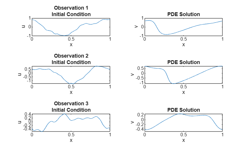
View some of the training data.

numPlots = 3;
gridSize = size(u0,2);
figure
tiledlayout(numPlots,2)
for i = 1:numPlots
    nexttile
    plot(linspace(0,1,gridSize),u0(i,:));
    title("Observation " + i + newline + "Initial Condition")
    xlabel("x")
    ylabel("u")

    nexttile
    plot(linspace(0,1,gridSize),u1(i,:));
    title("PDE Solution")
    xlabel("x")
    ylabel("v")
end

Three pairs of plots showing initial conditions (u vs. x) and corresponding PDE solutions (v vs. x) for observations 1, 2, and 3

Prepare Training Data

Split the training and test data using the trainingPartitions function, attached to the example as a supporting file. To access this function, open the example as a live script. Use 80% of the data for training, 10% for validation, and the remaining 10% for testing.

numObservations = size(u0,1);
[idxTrain,idxValidation,idxTest] = trainingPartitions(numObservations,[0.8 0.1 0.1]);
U0Train = u0(idxTrain,:);
U1Train = u1(idxTrain,:);

U0Validation = u0(idxValidation,:);
U1Validation = u1(idxValidation,:);
U0Test = u0(idxTest,:);

To reduce the amount of processing in the FNO, downsample the training and validation data so that it has a grid size of 1024.

gridSizeDownsampled = 1024;
downsampleFactor = floor(gridSize./gridSizeDownsampled);

U0Train = U0Train(:,1:downsampleFactor:end);
U1Train = U1Train(:,1:downsampleFactor:end);
U0Validation = U0Validation(:,1:downsampleFactor:end);
U1Validation = U1Validation(:,1:downsampleFactor:end);

The FNO requires the input data to have a channel that corresponds to the spatial coordinates (the grid). Create the grid and concatenate it with the input data.

xMin = 0;
xMax = 1;
xGrid = linspace(xMin,xMax,gridSizeDownsampled);

xGridTrain = repmat(xGrid, [numel(idxTrain) 1]);
xGridValidation = repmat(xGrid, [numel(idxValidation) 1]);

U0Train = cat(3,U0Train,xGridTrain);
U0Validation = cat(3,U0Validation,xGridValidation);

View the sizes of the training and validation sets. The first, second, and third dimensions are the batch, spatial, and channel dimensions, respectively.

size(U0Train)

ans = 1×3

    1638    1024    2

size(U0Validation)

ans = 1×3

    204    1024    2

Define Neural Network Architecture

Create the FNO network using the fnoNetwork function (since R2026b). The network consists of a lifting layer, multiple Fourier layers connected in series, and a projection layer.

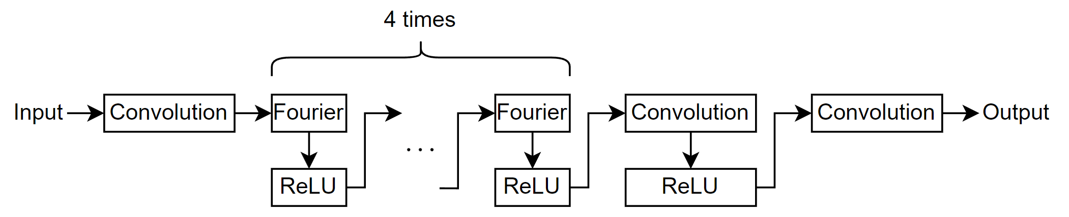
Diagram of the neural network of layers connected in series. From left to right, there is the input, convolution, four fourier-ReLU blocks, convolution, ReLU, convolution, and output.

Specify these options:

Use an input and output size that is consistent with the training predictors (the initial conditions) and targets (the PDE solution).
For a 1-D FNO network, specify that the data has one spatial dimension.
Specify four Fourier layers, with 16 Fourier modes, a hidden size of 64, and ReLU activations.

inputSize = size(U0Train,3);
outputSize = size(U1Train,3);

net = fnoNetwork(inputSize,outputSize, ...
    Dimension=1, ...
    NumFourierLayers=4, ...
    NumModes=16, ...
    HiddenSize=64, ...
    Activation="relu");

Before R2026b: Define the neural network architecture manually using a dlnetwork object.

Training Options

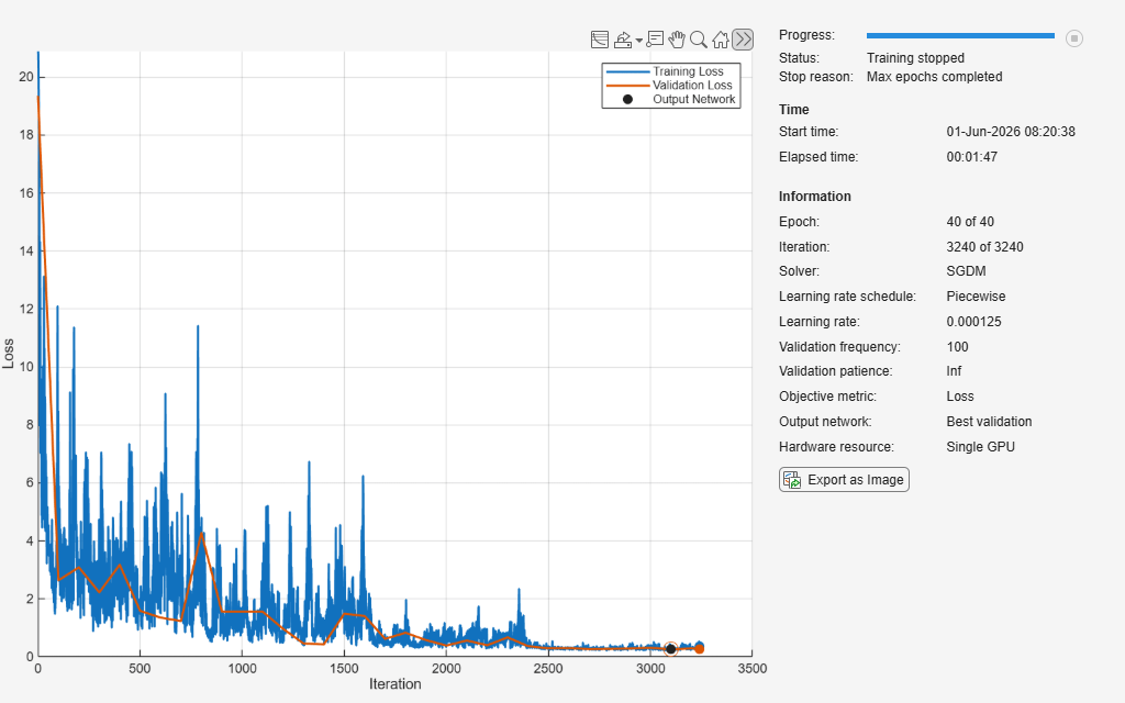
Specify the training options. Choosing among the options requires empirical analysis. To explore different training option configurations by running experiments, you can use the Experiment Manager app.

Train using the SGDM solver.
Train using a piecewise learning schedule, with an initial learning rate of 0.001 and a drop factor of 0.5.
Train for 40 epochs with a mini-batch size of 20.
Shuffle the data every epoch.
Because the input data has dimensions that correspond to batch, spatial, and channel dimensions, specify the input data format as "BSC".
Monitor the training progress in a plot.
Specify the validation data and validate the network every 100 iterations.
Disable the verbose output.

schedule = piecewiseLearnRate(DropFactor=0.5);

options = trainingOptions("sgdm", ...
    InitialLearnRate=1e-3, ...
    LearnRateSchedule=schedule, ...
    MaxEpochs=40, ...
    MiniBatchSize=20, ...
    Shuffle="every-epoch", ...
    InputDataFormats="BSC", ...
    Plots="training-progress", ...
    ValidationData={U0Validation,U1Validation}, ...
    ValidationFrequency=100, ...
    Verbose=false);

Define Relative $L_{2}$ Loss Function

Create the function relativeL2Loss, which takes the predictions and targets as input and returns the relative $L_{2}$ loss. The relative $L_{2}$ loss function is a variation of the $L_{2}$ loss function that accounts for scale by using the Euclidean norm of the difference between the predictions and targets and divides it by the Euclidean norm of the targets:

$R e l a t i v e L 2 (Y, T) = \sum_{n = 1}^{N} \frac{‖ T_{n} - Y_{n} ‖_{2}}{‖ T_{n} ‖_{2}}$

where:

$Y$ denotes the predictions.
$T$ denotes the targets.
$N$ denotes the number of observations.

To remove the formats from the dlarray inputs, use the stripdims function. Specify the dimension order as "SCB" so that the spatial dimension is first, for use with vecnorm.

function loss = relativeL2Loss(Y,T)

Y = stripdims(Y,"SCB");
T = stripdims(T,"SCB");

p = vecnorm(T-Y,2,1);
q = vecnorm(T,2,1);

loss = sum(p./q);

end

Train Network

Train the neural network using the trainnet function. Use the custom loss function relativeL2Loss. By default, the trainnet function uses a GPU if one is available. Using a GPU requires a Parallel Computing Toolbox™ license and a supported GPU device. For information on supported devices, see GPU Computing Requirements (Parallel Computing Toolbox). Otherwise, the function uses the CPU. To select the execution environment manually, use the ExecutionEnvironment training option.

net = trainnet(U0Train,U1Train,net,@relativeL2Loss,options);

Training progress plot showing training and validation loss decreasing over 3240 iterations across 40 epochs

Test Network

Test the prediction performance of the model by comparing the predictions on a held-out test set with the true labels and calculating the root mean squared error (RMSE).

Downsample the test data and concatenate the grid using the same steps as used for the training data.

xGridTest = repmat(xGrid, [numel(idxTest) 1]);

U0Test = U0Test(:,1:downsampleFactor:end);
U0Test = cat(3,U0Test,xGridTest);

U1Test = u1(idxTest,:);
U1Test = U1Test(:,1:downsampleFactor:end);

Test the neural network using the testnet function. By default, the testnet function uses a GPU if one is available. Otherwise, the function uses the CPU. To select the execution environment manually, use the ExecutionEnvironment argument of the testnet function.

rmseTest = testnet(net,U0Test,U1Test,"rmse",InputDataFormats="BSC")

rmseTest = 
0.0425

To evaluate the accuracy of the ZSSR, test the network using the test data without downsampling it.

xGridZSSR = linspace(xMin,xMax,gridSize);
xGridTestZSSR = repmat(xGridZSSR, [numel(idxTest) 1]);

U0TestZSSR = u0(idxTest,:);
U0TestZSSR = cat(3,U0TestZSSR,xGridTestZSSR);
U1TestZSSR = u1(idxTest,:);

rmseTestZSSR = testnet(net,U0TestZSSR,U1TestZSSR,"rmse",InputDataFormats="BSC")

rmseTestZSSR = 
0.0425

Make Predictions with New Data

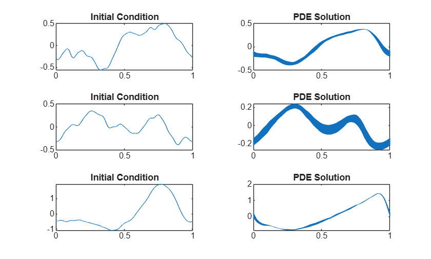
Load the new data. For example purposes, use the first three test observations.

dataNew = u0(idxTest(1:3),:);
numObservationsNew = size(dataNew,1);

Calculate the grid size and concatenate it with the data.

gridSizeNew = size(dataNew,2);
xGridNew = linspace(xMin,xMax,gridSizeNew);
xGridNew = repmat(xGridNew, [size(dataNew,1) 1]);
U0New = cat(3,dataNew,xGridNew);

Make predictions using the minibatchpredict function. By default, the minibatchpredict function uses a GPU if one is available. Otherwise, the function uses the CPU. To select the execution environment manually, use the ExecutionEnvironment option.

Y = minibatchpredict(net,U0New,InputDataFormats="BSC");

Visualize the predictions in a plot.

figure
tiledlayout(numObservationsNew,2)
for i = 1:numObservationsNew
    nexttile
    plot(xGridNew(i,:),dataNew(i,:))
    title("Initial Condition")

    nexttile
    plot(xGridNew(i,:),Y(i,:))
    title("PDE Solution")
end

Three pairs of plots showing initial conditions and predicted PDE solutions for three test observations, with high-resolution output from the trained FNO

References

Li, Zongyi, Nikola Kovachki, Kamyar Azizzadenesheli, Burigede Liu, Kaushik Bhattacharya, Andrew Stuart, and Anima Anandkumar. “Neural Operator: Graph Kernel Network for Partial Differential Equations.” arXiv, March 6, 2020. http://arxiv.org/abs/2003.03485.
Li, Zongyi, Nikola Kovachki, Kamyar Azizzadenesheli, Burigede Liu, Kaushik Bhattacharya, Andrew Stuart, and Anima Anandkumar. “Fourier Neural Operator for Parametric Partial Differential Equations,” 2020. https://openreview.net/forum?id=c8P9NQVtmnO.

Solve PDE Using Fourier Neural Operator

Load Training Data

Prepare Training Data

Define Neural Network Architecture

Training Options

Define Relative $L_{2}$ Loss Function

Train Network

Test Network

Make Predictions with New Data

References

See Also

Topics

Solve PDE Using Fourier Neural Operator

Load Training Data

Prepare Training Data

Define Neural Network Architecture

Training Options

Define Relative L2 Loss Function

Train Network

Test Network

Make Predictions with New Data

References

See Also

Topics

Define Relative $L_{2}$ Loss Function