Adaptive Line Enhancer (ALE)

Open Script

This example shows how to apply adaptive filters to signal separation using a structure called an adaptive line enhancer (ALE). In adaptive line enhancement, a measured signal x(n) contains two signals, an unknown signal of interest v(n), and a nearly-periodic noise signal eta(n).

The goal is to remove the noise signal from the measured signal to obtain the signal of interest.

Author(s): Scott C. Douglas

Loading the Signal of Interest

We'll first load in a signal of interest, a short clip from Handel's Hallelujah chorus.

audioReader = dsp.AudioFileReader('handel.ogg','SamplesPerFrame',44100);
timeScope = timescope('SampleRate',audioReader.SampleRate,...
    'YLimits',[-1,1],'TimeSpanSource','property','TimeSpan',1);

while ~isDone(audioReader)
    x = audioReader() / 2;
    timeScope(x);
end

Listening to the Sound Clip

You can listen to the signal of interest using the audio device writer.

release(audioReader);
audioWriter = audioDeviceWriter;
while ~isDone(audioReader)
    x = audioReader() / 2;
    audioWriter(x);
end

Generating the Noise Signal

Let's now make a periodic noise signal--a sinusoid with a frequency of 1000 Hz.

sine = dsp.SineWave('Amplitude',0.5,'Frequency',1000,...
    'SampleRate',audioReader.SampleRate,...
    'SamplesPerFrame',audioReader.SamplesPerFrame);

Now let's plot 10 msec of this sinusoid above. It shows 10 periods in 10 msec, just as it should.

eta = sine();
Fs  = sine.SampleRate;
plot(1/Fs:1/Fs:0.01,eta(1:floor(0.01*Fs)));
xlabel('Time [sec]');
ylabel('Amplitude');
title('Noise Signal, eta(n)');

Listening to the Noise

The periodic noise is a pure tone. The following code plays one second (one frame of 44100 samples) of the noise signal.

eta = sine();
release(audioWriter);
audioWriter(eta);

Measured Signal

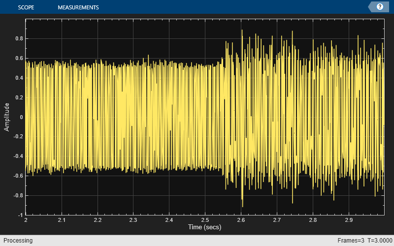
The signal that we actually measure is the sum of these two signals, and we call this signal s(n). A plot of s(n) shows that the envelope of the music signal is largely obscured. Listening to a 3-second clip from the measured signal, the noise is clearly prominent...

release(audioReader);
release(timeScope);
release(audioWriter);
count = 1;
while count < 4
    s = (audioReader() / 2) + sine();
    timeScope(s);
    audioWriter(s);
    count = count + 1;
end

Adaptive Filter Configuration

An adaptive line enhancer (ALE) is based on the straightforward concept of linear prediction. A nearly-periodic signal can be perfectly predicted using linear combinations of its past samples, whereas a non-periodic signal cannot. So, a delayed version of the measured signal s(n-D) is used as the reference input signal x(n) to the adaptive filter, and the desired response signal d(n) is made equal to s(n). The parameters to choose in such a system are the signal delay D and the filter length L used in the adaptive linear estimate. The amount of delay depends on the amount of correlation in the signal of interest. Since we don't have this signal (if we did, we wouldn't need the ALE!), we shall just pick a value of D=100 and vary it later. Such a choice suggests that samples of the Hallelujah Chorus are uncorrelated if they are more than about 12 msec apart. Also, we'll choose a value of L=32 for the adaptive filter, although this too could be changed.

D = 100;
delay = dsp.Delay(D);

Finally, we shall be using some block adaptive algorithms that require the lengths of the vectors for x(n) and d(n) to be integer multiples of the block length. We'll choose a block length of N=49 with which to begin.

Block LMS

The first algorithm we shall explore is the Block LMS algorithm. This algorithm is similar to the well-known least-mean-square (LMS) algorithm, except that it employs block coefficient updates instead of sample-by-sample coefficient updates. The Block LMS algorithm needs a filter length, a block length N, and a step size value mu. How do we pick mu? Let's start with a value of mu = 0.0001 and refine it shortly.

L  = 32;
N  = 49;
mu = 0.0001;
blockLMSFilter = ...
    dsp.BlockLMSFilter('Length',L,'StepSize',mu,'BlockSize',N);

Running the Filter

The output signal y(n) should largely contain the periodic sinusoid, whereas the error signal e(n) should contain the musical information, if we've done everything right. Since we have the original music signal v(n), we can plot e(n) vs. v(n) on the same plot shown above along with the residual signal e(n)-v(n). It looks like the system is converged after about 5 seconds of adaptation with this step size. The real proof, however, is obtained by listening;

release(audioReader);
release(timeScope);
release(audioWriter);
while ~isDone(audioReader)
    x = audioReader() / 2;
    s = x + sine();
    d = delay(s);
    [y,e] = blockLMSFilter(s,d);
    timeScope(e);
    audioWriter(e);
end

Notice how the sinusoidal noise decays away slowly. This behavior is due to the adaptation of the filter coefficients toward their optimum values.

FM Noise Source

Now, removing a pure sinusoid from a sinusoid plus music signal is not particularly challenging if the frequency of the offending sinusoid is known. A simple two-pole, two-zero notch filter can perform this task. So, let's make the problem a bit harder by adding an FM-modulated sinusoidal signal as our noise source.

eta = 0.5 * sin(2*pi*1000/Fs*(0:396899)' + 10*sin(2*pi/Fs*(0:396899)'));
signalSource = dsp.SignalSource(eta,...
    'SamplesPerFrame',audioReader.SamplesPerFrame,...
    'SignalEndAction','Cyclic repetition');
release(audioReader);
release(timeScope);
release(audioWriter);
while ~isDone(audioReader)
    x = audioReader() / 2;
    s = x + signalSource();
    timeScope(s);
    audioWriter(s);
end

The "warble" in the signal is clearly audible. A fixed-coefficient notch filter won't remove the FM-modulated sinusoid. Let's see if the Block LMS-based ALE can. We'll increase the step size value to mu=0.005 to help the ALE track the variations in the noise signal.

mu = 0.005;
release(blockLMSFilter);
blockLMSFilter.StepSize = mu;

Running the Adaptive Filter

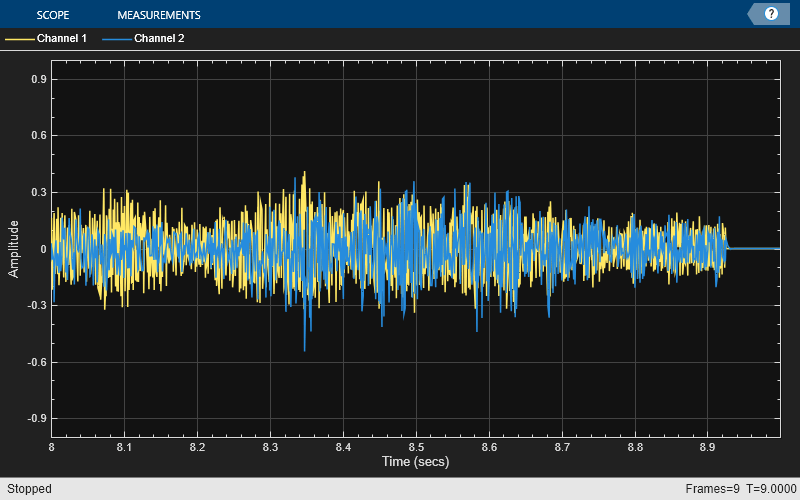
We now filter the noisy music signal with the adaptive filter and compare the error to the noiseless music signal.

release(audioReader);
release(timeScope);
release(audioWriter);
while ~isDone(audioReader)
    x = audioReader() / 2;
    s = x + signalSource();
    d = delay(s);
    [y,e] = blockLMSFilter(s,d);
    timeScope([x,e]);
    audioWriter(e);
end

release(audioReader);
release(timeScope);
release(audioWriter);