Streaming Power Spectrum Estimation Using Welch's Method
Compute the power spectrum estimate of a time-domain input signal using the Spectrum Estimator block. The block uses one of the following methods to compute the power spectrum estimate:
Welch's method of averaged modified periodograms
Filter bank method
This example uses the Welch's method of averaged modified periodograms. For an example that uses the filter bank-based spectrum estimation method, see High Resolution Spectral Analysis in MATLAB. The same example also shows the comparison between the filter bank estimator and the Welch-based spectral estimator. Generally, filter bank-based spectrum estimation yields better resolution with less spectral leakage, more accurate peaks and a more accurate noise floor.
For more details on algorithm of these two methods, see the 'Algorithms' section in the Spectrum Estimator block.
The Spectrum Estimator block is useful if you need direct access to the estimated spectrum (rather than just visualize it). The output power spectrum may be used as an input to other blocks in your model, or may be logged to the workspace for post-processing. To visualize the spectra, use the Spectrum Analyzer scope block.
Welch's Method of Averaged Modified Periodograms
In the Welch method, the input time-domain data is partitioned into data segments based on the selected window length and overlap percentage. This stage is implemented using a Buffer block. A window is applied to each segment, and then an averaged periodogram is computed based on the windowed sequences. This stage is implemented using a dsp.SpectrumEstimator System object™. The length of the data segments and the choice of the window determine the estimate's resolution bandwidth (RBW), which is the smallest positive frequency that can be resolved in the power spectral estimate.
Specifying Window Length
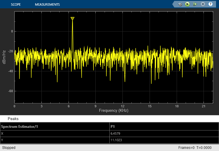
The dspstreamingwelch model shown below uses a Welch Spectrum Estimator block to estimate the spectrum of a noisy chirp signal sampled at 44100 Hz. The power spectrum estimate is displayed using an Array Plot scope. The peak value of the spectrum, as well as the frequency at which the peak occurs, are detected and displayed on the scope. The estimate's RBW is also displayed. Moreover, a Spectrum Analyzer scope block is included for comparison and validation purposes.

The block's frequency resolution method is set to Welch. The data is windowed using a Chebyshev window with a sidelobe attenuation of 60 dB. The frequency range is one-sided. In this case, the length of the spectrum estimate is  and is computed over the interval [0 Hz,22050 Hz]. The Sample Increment property of the Array Plot scope is accordingly set to
  , where the increment is divided by 1000 to scale the frequency units to kHz. You can access the scope's Sample Increment property by opening its Settings in the Scope tab.
The resolution bandwidth is given by:

where,
 is the window length in the Spectrum Estimator block
 is a function that computes the equivalent noise bandwidth of the window.
 is the sidelobe attenuation of the Chebyshev window.
 is the sample rate.
Using the values in the Spectrum Estimator block, the RBW is equal to 65.38 Hz.
Set RBW (Hz) to 65.38 Hz in the Scope tab of the Spectrum Analyzer toolstrip. The two blocks give the same peak measurements.


Specifying Non-Zero Overlap
The model in the previous section had zero-overlap. In the dspstreamingwelch_overlap model, we use an overlap of 50%. The RBW is 65.38 Hz, With a window length of 1024 and an overlap percentage of 50%, 512 input samples are required to form a new data segment. Since the input data is of length 1024, each new data frame yields two new periodograms, and the Spectrum Analyzer block output port runs at a rate twice as fast as the input port.
Note that the Spectrum Estimator block does not have zero latency in this case. The first spectrum estimate output is based on the buffer's initial condition, which is equal to eps. In order to match the spectrum and measurements of the Spectrum Analyzer scope, we therefore insert a delay block at the input of the Spectrum Analyzer.
The results of the Spectrum Analyzer and Welch estimate block may be validated by simulating the model.


Specifying RBW
In the dspstreamingwelch_rbw model, the RBW (Hz) is set to Auto. In this mode, the resolution bandwidth is chosen such that there are 1024 RBW intervals over the specified frequency Span. Since the span in this case is 22050 HZ, the RBW is 21.53 Hz.
The window length used to buffer the data is iteratively computed to yield the desired RBW. The window length in this case is equal to 3073. To verify this value, we can compute the RBW that results from this window length:

Note that a Hann window is used in this model. In this case, the FFT length, NFFT, is odd and equal to 3073 (the window length). Since the frequency range is one-sided, the spectrum estimate is of length (NFFT + 1)/2 and is computed over the interval [0,44100/2). The Sample Increment property of the Array Plot scope is set to  KHz.
KHz.
Again, the results of the Spectrum Analyzer and Welch estimate block can be validated by simulating the model.


References
[1] Hayes, Monson H. Statistical Digital Signal Processing and Modeling Hoboken, NJ: John Wiley & Sons, 1996.