Forecast a Regression Model with Multiplicative Seasonal ARIMA Errors

This example shows how to forecast a multiplicative seasonal ARIMA model using forecast. The response series is monthly international airline passenger numbers from 1949 to 1960.

Load the airline and recessions data sets. Transform the response.

load Data_Airline
load Data_Recessions
y = log(DataTimeTable.PSSG);

Construct the predictor (X), which determines whether the country was in a recession during the sampled period. A 0 in row t means the country was not in a recession in month t, and a 1 in row t means that it was in a recession in month t.

X = zeros(numel(dates),1); % Preallocation
for j = 1:size(Recessions,1)
    X(dates >= Recessions(j,1) & dates <= Recessions(j,2)) = 1;
end

Define index sets that partition the data into estimation and forecast samples.

nSim = 60; % Forecast period
T = length(y);
estInds = 1:(T-nSim);
foreInds = (T-nSim+1):T;

Estimate the regression model with multiplicative seasonal ARIMA} $$(0,1,1)\times (0,1,1{)}_{12}$$ errors:

$$y_t=X_t\beta +u_t$$

$$(1-L)(1-L^{12})u_t=(1+BL)(1+B_{12}{L}^{12}){\epsilon }_t$$

Set the regression model intercept to 0 since it is not identifiable in a model with integrated errors.

Mdl = regARIMA('D',1,'Seasonality',12,'MALags',1,'SMALags',12,...
    'Intercept',0);
EstMdl = estimate(Mdl,y(estInds),'X',X(estInds)); 

 
    Regression with ARIMA(0,1,1) Error Model Seasonally Integrated with Seasonal MA(12) (Gaussian Distribution):
 
                   Value      StandardError    TStatistic      PValue  
                 _________    _____________    __________    __________

    Intercept            0              0           NaN             NaN
    MA{1}         -0.35662        0.10393       -3.4312      0.00060088
    SMA{12}       -0.67729        0.11294       -5.9972      2.0077e-09
    Beta(1)      0.0015098       0.020533       0.07353         0.94138
    Variance     0.0015198     0.00021411        7.0983      1.2632e-12

Use the estimated coefficients of the model (contained in EstMdl), to generate MMSE forecasts and corresponding mean square errors over a 60-month horizon. Use the observed series as presample data. By default, forecast infers presample innovations and unconditional disturbances using the specified model and observations.

[YF,YMSE] = forecast(EstMdl,nSim,'X0',X(estInds),...
    'Y0',y(estInds),'XF',X(foreInds));
ForecastInt = [YF,YF] + 1.96*[-sqrt(YMSE), sqrt(YMSE)];
fh = DataTimeTable.Time(foreInds);

figure
h1 = plot(DataTimeTable.Time,y);
title('{\bf Forecasted Monthly Passenger Totals}')
hold on
h2 = plot(fh,YF,'Color','r','LineWidth',2);
h3 = plot(fh,ForecastInt,'k--','LineWidth',2);
legend([h1,h2,h3(1)],'Observations','MMSE Forecasts',...
    '95% MMSE Forecast Intervals','Location','NorthWest')
axis tight
hold off

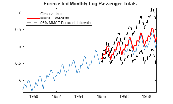
The regression model with SMA errors seems to forecast the series well, albeit slightly overestimating. Since the error process is nonstationary, the forecast intervals widen as time increases.

Compare the MMSE forecasts to Monte Carlo forecasts by simulating 500 sample paths from EstMdl over the forecast horizon.

[e0,u0] = infer(EstMdl,y(estInds),'X',X(estInds));
rng(5);
numPaths = 500;
ySim = simulate(EstMdl,nSim,'numPaths',numPaths,...
    'E0',e0,'U0',u0,'X',X(foreInds));
meanYSim = mean(ySim,2);
ForecastIntMC = [prctile(ySim,2.5,2),prctile(ySim,97.5,2)];

figure
h1 = plot(fh,y(foreInds));
title('{\bf Forecasted Monthly Passenger Totals}')
hold on
h2 = plot(fh,YF,'Color',[0.85,0.85,0.85],...
    'LineWidth',4);
h3 = plot(fh,ForecastInt,'--','Color',...
    [0.85,0.85,0.85],'LineWidth',4);
h4 = plot(fh,meanYSim,'k','LineWidth',2);
h5 = plot(fh,ForecastIntMC,'k--','LineWidth',2);
legend([h1,h2,h3(1),h4,h5(1)],'Observations',...
    'MMSE Forecasts','95% MMSE Forecast Intervals',...
    'Monte Carlo Forecasts','95% Monte Carlo Forecast Intervals',...
    'Location','NorthWest')
axis tight
hold off

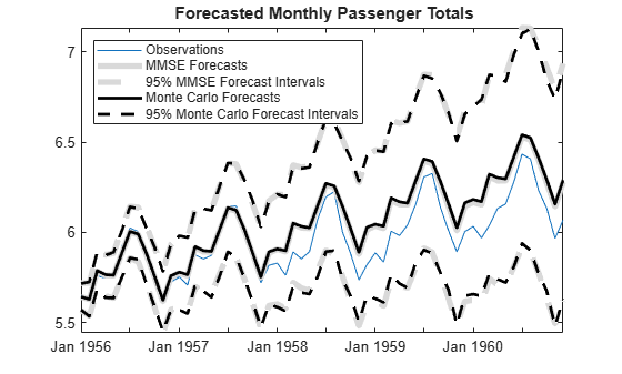
The MMSE forecasts and Monte Carlo mean forecasts are virtually indistinguishable. However, there are slight discrepancies between the theoretical 95% forecast intervals and the simulation-based 95% forecast intervals.