Compare Numerical Response of Sum Block and Sum in MATLAB Function Block
This example shows how to generate simulation inputs and use them to exercise a model over its full operating range. In this example, generate test data to simulate a model and compare the numerical response of the Sum block, and sum implemented in a MATLAB® Function block in the ex_testsum model.
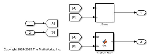
Open the model.
model = 'ex_testsum';
open_system(model);
Specify Data Attributes and Generate Data
Use the fixed.DataSpecification object to specify input data attributes. In this example, create two DataSpecification objects, one with a double-precision data type, and the other using a single-precision data type. The interval of values generated by the first object is from 1 to 64, and the interval of values generated by the second is from 1 to 32.
dataspec1 = fixed.DataSpecification('double', 'Intervals', {1 64});
dataspec2 = fixed.DataSpecification('single', 'Intervals', {1 32});
The DataGenerator object generates combinations of numerically-rich values. To use the output data in a Simulink® model, set the format of the output to 'timeseries'.
datagen = fixed.DataGenerator;
datagen.DataSpecifications = {dataspec1, dataspec2};
[tsdata1, tsdata2] = outputAllData(datagen, 'timeseries');
Set Up Model and Simulate
Apply the attributes of the DataSpecification objects to the Inport blocks in the model.
set_param('ex_testsum/In1',...
    'OutDataTypeStr',dataspec1.DataTypeStr,...
    'SignalType',dataspec1.Complexity,...
    'PortDimensions',['[' num2str(dataspec1.Dimensions) ']'])
set_param('ex_testsum/In2',...
    'OutDataTypeStr',dataspec2.DataTypeStr,...
    'SignalType',dataspec2.Complexity,...
    'PortDimensions',['[' num2str(dataspec2.Dimensions) ']'])
Load the generated timeseries data into the model and simulate.
set_param(model, 'LoadExternalInput', 'on',...
    'ExternalInput', 'tsdata1, tsdata2',...
    'StopTime', string(tsdata1.Time(end)));

simout = sim(model);

Visualize Output
Visualize the output of the simulation, and compare the numerical behavior of the two implementations of the sum operation.
Get the unique values in the generated data for each set of data.
[x, y] = datagen.getUniqueValues;
d = abs(simout.yout{1}.Values.Data - simout.yout{2}.Values.Data);
X = reshape(tsdata1.Data, numel(x), []);
Y = reshape(tsdata2.Data, numel(x), []);
D = reshape(d, numel(x), []);
Plot the difference between outputs as a function of the input values.
figure;
surf(X, Y, D, 'EdgeColor', 'none');
grid on;
view(2);
axis tight;
xlabel('In1');
ylabel('In2');
colorbar;
title('abs(MATLAB Function block output - Sum block output)');
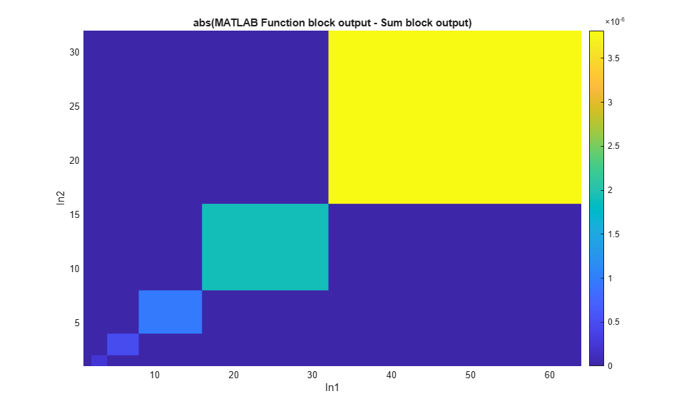
From the plot, you can see that the difference between the two implementations increases as the values of the numeric inputs get larger. This difference is due to the difference in the data type of the accumulator in the two implementations.
Compare Numerical Response with Single-Precision Accumulator
The Accumulator Data Type parameter of the Sum block is set to Inherit: Inherit via internal rule. In this case, the data type used for the accumulator is a double-precision floating-point type. Set the Accumulator data type to single and compare the output again.
set_param([model,'/Sum'], 'AccumDataTypeStr', 'single')
simout = sim(model);
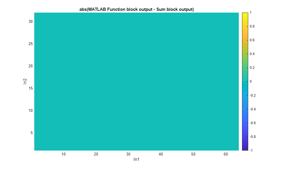
Visualize the output. When the accumulator type of the Sum block is set to single, the implementations return the same result at all values.
[x, y] = datagen.getUniqueValues;
d = abs(simout.yout{1}.Values.Data - simout.yout{2}.Values.Data);
X = reshape(tsdata1.Data, numel(x), []);
Y = reshape(tsdata2.Data, numel(x), []);
D = reshape(d, numel(x), []);
figure;
surf(X, Y, D, 'EdgeColor', 'none');
grid on;
view(2);
axis tight;
xlabel('In1');
ylabel('In2');
colorbar;
title('abs(MATLAB Function block output - Sum block output)');
