Optimize the Fixed-Point Data Types of a System Using the Fixed-Point Tool
This example shows how to define simulation scenarios and use the Fixed-Point Tool to collect ranges by running simulations using these scenarios. You can then use the Fixed-Point Tool to optimize the fixed-point data types of the system.
During the optimization, the software establishes a baseline by simulating the original
model. It then constructs different fixed-point versions of your model and runs simulations to
determine the behavior using the new data types. The optimization selects the model that
minimizes the objective function while also meeting the specified behavioral constraints.
Including a Simulink.SimulationInput object in the setup allows you to
define additional simulation scenarios to consider during the optimization. A comprehensive
set of input signals can help to ensure that the full operating range of your design is
exercised during the optimization process.
Open Model and Define Simulation Scenarios
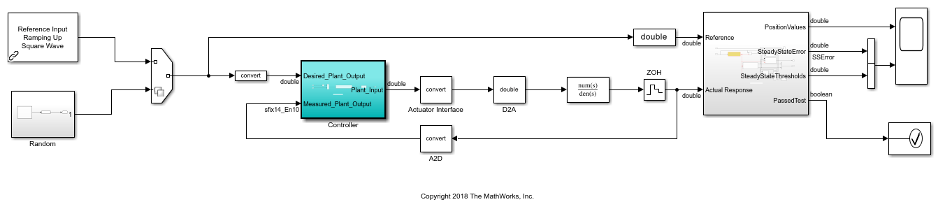
Open the model. In this example, you optimize the data types of the Controller subsystem. The model is set up to use either a ramp input, or a random input.
model = 'ex_controllerHarness';
open_system(model)
Create a Simulink.SimulationInput object that contains the different scenarios. Use both the ramp input as well as four different seeds for the random input.
si = Simulink.SimulationInput.empty(5, 0);

% scan through 4 different seeds for the random input
rng(1);
seeds = randi(1e6, [1 4]);

for sIndex = 1:length(seeds)
    si(sIndex) = Simulink.SimulationInput(model);
    si(sIndex) = si(sIndex).setVariable('SOURCE', 2); % SOURCE == 2 corresponds to the random input
    si(sIndex) = si(sIndex).setBlockParameter([model '/Random/uniformRandom'], 'Seed', num2str(seeds(sIndex))); % scan through the seeds
    si(sIndex) = si(sIndex).setUserString(sprintf('random_%i', seeds(sIndex)));
end

% setting SOURCE == 1 corresponds to the ramp input
si(5) = Simulink.SimulationInput(model);
si(5) = si(5).setVariable('SOURCE', 1);
si(5) = si(5).setUserString('Ramp');
Prepare System for Conversion
To optimize the data types in the mode, use the Fixed-Point Tool.
In the Apps gallery of the
ex_controllerHarnessmodel, select Fixed-Point Tool.In the Fixed-Point Tool, under New workflow, select
Optimized Fixed-Point Conversion.Under System Under Design (SUD), select the subsystem for which you want to optimize the data types. In this example, select
Controller.Under Range Collection Mode, select Simulation Ranges as the range collection method.
Under Simulation Inputs, you can specify
Simulink.SimulationInputobjects to exercise your design over its full operating range. In this example, use the simulation scenarios you defined. Set Simulation Inputs tosi.You can specify tolerances for any signal in the model with signal logging enabled in the table under Signal Tolerances. In this example, the Signal Tolerances section indicates that the model contains no logged signals. Because this model uses an Assertion block from the Model Verification library to verify the numerical behavior of the system during optimization, specifying signal tolerances is optional. For more information, see Specify Behavioral Constraints.
If you have an
fxpOptimizationOptionsobject saved from a prior command line optimization, for example if you previously optimized data types in this model following the example Optimize Data Types Using Multiple Simulation Scenarios, you can import thefxpOptimizationOptionsobject under the Advanced Options section. The Setup pane and toolstrip Settings menu will be updated with the imported values. If an optimization options object is not imported, the default values are used unless otherwise changed manually in the Fixed-Point Tool. For this example, you will specify the settings manually in the app.In the toolstrip, click Prepare. The Fixed-Point Tool checks the system under design for compatibility with the conversion process and reports any issues found in the model. When possible, the Fixed-Point Tool automatically changes settings that are not compatible. For more information, see Use the Fixed-Point Tool to Prepare a System for Conversion.
Optimize Data Types in the Fixed-Point Tool
To specify settings to use during the optimization, in the toolstrip, click Optimization Options.
In this example, use the following settings.
Set Allowable Word Lengths to
[2:32].This setting defines the word lengths that can be used in your optimized system. Use this setting to target the neighborhood search of the optimization process. The final result of the optimization uses word lengths in the intersection of this setting and word lengths compatible with hardware constraints specified in the Hardware Implementation pane of your model.
Set Max Iterations to
3e2.This setting specifies the maximum number of iterations to perform in the optimization. The optimization process iterates through different solutions until it finds an ideal solution, reaches the maximum number of iterations, or reaches another stopping criteria.
Set Patience to
50.This setting defines the maximum number of iterations where no new best solution is found. The optimization continues as long as the algorithm continues to find new best solutions.
Set Objective Function to Bit Width Sum. Using this setting instructs the optimization to minimize the total bit width of the final design while meeting the specified constraints.
For more information about optimization settings, see
fxpOptimizationOptions.To optimize the data types in the model according to the specified settings, click Optimize Data Types.
During the optimization process, the software analyzes ranges of objects in your system under design and the constraints specified in the settings to apply heterogeneous data types to your system while minimizing the objective function. Details about the optimization process are printed to the Optimization Details pane in the Fixed-Point Tool.
You can stop the optimization solver before the optimization search is complete by clicking Stop in the toolstrip of the Fixed-Point Tool. To resume optimization from where you left off, click Optimize Data Types to restart the optimization solver.
Perform Neighborhood Searchmust be activated to resume optimization. You can also choose to modify the stopping criteria for the optimization solver, includingMax Iterations,Max Time (sec), andPatience (iterations). This can help to quickly narrow down a large optimization search space.
Examine Results
When the optimization completes, the Fixed-Point Tool displays the solutions found during the optimization process in a table. The first solution in the table corresponds to the solution with the lowest cost (smallest total bit width). The solutions are also plotted in a scatter chart that compares the cost and maximum difference of each solution to help you visualize the tradeoff between accuracy and cost-efficiency for each solution. When you select any solution in the table, the solution is highlighted in the scatter chart.
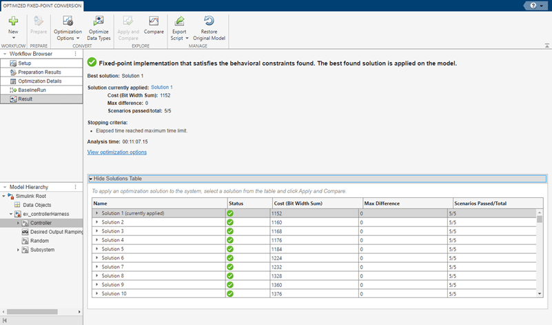
To view the settings that were used for optimization, in the Result pane, click View optimization options.
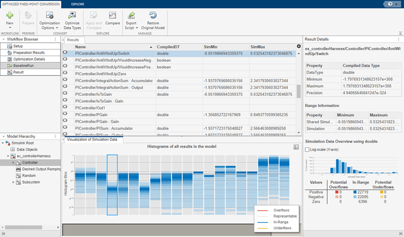
To inspect the ranges that were collected for objects in your model during the optimization process, in the Workflow Browser pane, select BaselineRun.
The Fixed-Point Tool displays a summary of the ranges of objects in your model and histograms of the bits used by each object. Each column in the Visualization of Simulation Data pane represents a histogram for one object in your model. Each bin in a histogram corresponds to a bit in the binary word.
Selecting a column highlights the corresponding model object in the Results spreadsheet of the Fixed-Point Tool and populates the Result Details pane with more detailed information about the selected result.
You can use the data type visualization to see a summary of the ranges of objects in your model and to spot sources of overflow, underflows, and inefficient data types. Using the Explore tab of the Fixed-Point Tool, you can sort and filter results in the tool based on additional criteria.
Apply Optimized Data Types to the Model
To apply the optimized data types to the model, in the solutions table, select the solution that you want to apply. In the Explore section of the toolstrip, click Apply and Compare. The Fixed-Point Tool applies the selected solution that contains optimized fixed-point data types to the model and opens the Simulation Data Inspector.
In this example, the best solution, Solution 1, is automatically applied to the model.
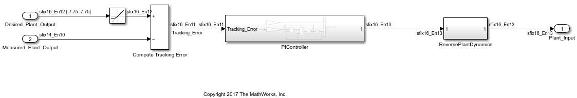
In the Controller subsystem, you can see the applied, optimized fixed-point data types.
Tip
The Fixed-Point Tool uses the Simulation Data Inspector tool plotting capabilities that enable you to plot logged signals for graphical analysis. Because this model does not contain any logged signals, the Compare button remains disabled in this example. To compare results of data type optimization using the Simulation Data Inspector, log one or more signals in your model.
Export Optimization Workflow Steps to a MATLAB Script
After optimizing data types in the Fixed-Point Tool, you can choose to export
optimization workflow steps to a MATLAB® script. This allows you to save the current optimization workflow steps and
continue data type optimization using fxpopt at
the command line.
In the toolstrip, click Export Script. The Fixed-Point Tool
exports a script called fxpOptimizationScript.m to the current working
directory:
model = 'ex_controllerHarness';

sud = 'ex_controllerHarness/Controller';

options = fxpOptimizationOptions();

options.MaxIterations = 300; % Maximum number of iterations to perform.

options.Patience = 50; % Maximum number of iterations where no new best solution is found.

options.AllowableWordLengths = 2:32; % Word lengths that can be used in your optimized system under design.

savedOptions = load('fxpOptimizationScript');

options.AdvancedOptions.SimulationScenarios = savedOptions.simulationScenarios;

result = fxpopt(model, sud, options);

explore(result);
The Simulink.SimulationInput object, si, used
during optimization is exported to a MAT file called
fxpOptimizationScript.mat.