Grid-based Tracking in Urban Environments Using Multiple Lidars in Simulink
This example shows how to track moving objects with multiple lidars using a grid-based tracker in Simulink. You use the Grid-Based Multi Object Tracker Simulink block to define the grid-based tracker. This Grid-based tracker uses dynamic occupancy grid map as an intermediate representation of the environment. This example closely follows the Grid-Based Tracking in Urban Environments Using Multiple Lidars MATLAB® example.
Overview of the model
![]()
The model is composed of three parts:
Scenario and Sensor SimulationVisualization
Scenario and Sensor Simulation
![]()
The Scenario Reader block reads a drivingScenario (Automated Driving Toolbox) object from workspace and generates Actors and Ego vehicle position data as Simulink.Bus (Simulink) objects. The subsystem Sensor Model and Transformation helps to generate multiple lidar sensor data and transform that data into a high-resolution sensor data. The HelperConcatenateSensorData block is implemented using a MATLAB Function (Simulink) block. Code for this block is defined in the HelperSensorData file. This block groups the data received from Sensor Model and Transformation subsystem, which is used as an input to the tracker block.
Sensor Model and Transformation
![]()
The HelperLidarSensorConfigurations block generates real time lidar sensors configuration with the help of Runtime objects obtained from the Scenario Reader and Lidar Point Cloud Generator blocks. These sensor configurations allow you to specify the mounting of each sensor with respect to the tracking coordinate frame. The sensor configurations also allow you to specify the detection limits - field of view and maximum range - of each sensor. As the sensors move in the scenario system, their configurations must be updated each time by specifying the configurations as an input to the tracker block. The HelperConvertLidarToSensorData block is implemented using a MATLAB Function (Simulink) block. Code for this block is defined in the HelperLidarToSensorData file. This block transforms the data coming from lidar sensors and sensor configurations Runtime object from the HelperLidarSensorConfigurations block into a high resolution sensor data.
The scenario used in this example was created using the Driving Scenario Designer (Automated Driving Toolbox) app and then exported to a MATLAB® function. The scenario represents an urban intersection scene and contains a variety of objects including pedestrians, bicyclists, cars, and trucks. The ego vehicle is equipped with six homogeneous lidars, each with a horizontal field of view of 90 degrees and a vertical field of view of 40 degrees. Each lidar has 32 elevation channels and has a resolution of 0.16 degrees in azimuth. Under this configuration, each lidar sensor outputs approximately 18,000 points per scan. The configuration of each sensor is shown here.
Grid-Based Multi Object Tracker
You use the Grid-Based Multi Object Tracker block to implement the tracking algorithm to track dynamic objects in the scene. You define all the parameters in the block mask based on the scenario requirement. To visualize the dynamic grid map, make sure you select the Enable dynamic grid map visualization parameter on the visualization tab of the tracker block.
Visualization
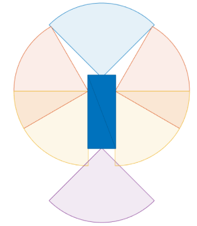
The visualization used for this example is defined using a helper class, HelperVisualization a MATLAB System (Simulink) block, attached with this example. In the step call of visualization block make sure you set the "Parent" property to the current axes. This allows you to visualize the dynamic grid map on the current figure axes. The color disc classifies the motion of the grid cells object. You can see that the grid cells motion in the positive x-direction are classified with red color, objects moving in the negative x-direction are classified with the blue color, objects moving in the negative y-direction are classified with purple and objects moving in the positive y-direction are classified with light-green color. The Visualization contains three parts:
Ground truth - Front View: This panel shows the front-view of the ground truth using a chase plot from the ego vehicle. To emphasize dynamic actors in the scene, the static objects are shown in gray.
Lidar Views: These panels show the point cloud returns from each sensor.
Grid-based tracker: This panel shows the grid-based tracker outputs. The tracks are shown as boxes, each annotated by their identity. The tracks are overlaid on the dynamic grid map. The colors of the dynamic grid cells are defined according to the color wheel, which represents the direction of motion of in the scenario frame. The static grid cells are represented in grayscale according to their occupancy. The degree of grayness denotes the probability that the space occupied by the grid cell is free. The positions of the tracks are shown in the ego vehicle coordinate system, while the velocity vector corresponds to the velocity of the track in the scenario frame.
![]()
Results and Analysis
You can analyze the performance of the tracker based on the visualization results. The Grid-based tracker panel shows the estimated dynamic map as well as the estimated tracks of the objects. It also shows the configurations of sensors, which are mounted on the ego vehicle and shown as blue circular sectors. Notice that the grey area shown in the dynamic grid map is not observable from any of the ego vehicle sensors since the view direction is blocked. You can also find that the tracks are only extracted from the dynamic cells and hence the tracker is able to filter out static objects.
Summary
In this example you learned how to construct a grid-based multi object tracking system and how to track and visualize dynamic objects in a complex urban driving environment in Simulink.