Understand and Analyze JIPDA Smoother Algorithm

Open Live Script

This example demonstrates the JIPDA smoothing algorithm and presents a graphical user interface (GUI) to analyze the intermediate results of the smoothing process. This example is an extension to the Introduction to JIPDA Smoothing example.

Introduction

As shown in the Introduction to JIPDA Smoothing example, the JIPDA smoother is an offline multi-object tracking algorithm. At each time instant of observations, the JIPDA smoother estimates probabilistic data association weights between tracks and measurements. The key difference between a JIPDA smoother and a JIPDA tracker is that the smoother can use information from future time instants to estimate the data association. In this example, you use the same scenario as shown in the Introduction to JIPDA Smoothing example to study the intermediate steps of the smoother by using a graphical user interface (GUI) based analysis tool.

Analysis App

To perform iterative analysis of the JIPDA smoother for interpreting the intermediate results of the smoothing algorithm, specify the AnalysisFcn property of the smoother using your custom function. Designed using App Designer, the app used in this example allows you to visualize, inspect, and interact with the intermediate results provided by the smoother. The required files for the app are attached in a zip file named AnalysisApp.zip.

% Unzip Analysis App
appExists = exist('AnalysisApp.mlapp','file');
if ~appExists
    unzip('AnalysisApp.zip');
    oldPath = addpath(genpath(fullfile(pwd,'AnalysisApp')));
end

You set up the problem in the Problem Setup section of the app. First, you specify the variable name of recorded detections and the smootherJIPDA object available in the MATLAB base workspace. You also specify the time stamps at which the smoother outputs smoothed track estimate. You can further select if the smoother should run in code generation mode to accelerate the simulation speed. The code generation mode requires a MATLAB® Coder™ license. Code generation requires an initial setup time to generate code but can accelerate the smoother when running on large datasets.

% Create data
[detectionLog, timestamps] = createSimpleScenarioData();

% Create smoother
smoother = smootherJIPDA;

% Start the App
app = AnalysisApp;

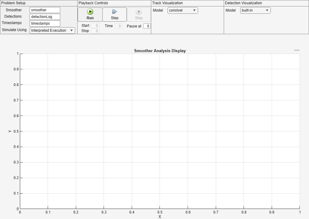
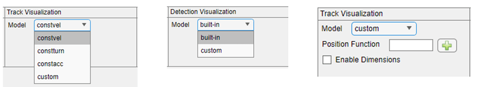
Next, you set up models for visualizing tracks and detections. By default, the application supports built-in models for both detections and tracks. Alternatively, you can specify a custom model by writing a simple parsing function for tracks or detections.

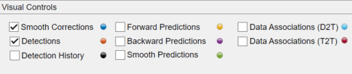
The Playback Controls section of the app allows you to play, pause, step, and stop simulation. You can also choose to pause at a specified time stamp. During simulation, the application allows you to control the information plotted on the figure by using these visual controls shown below.

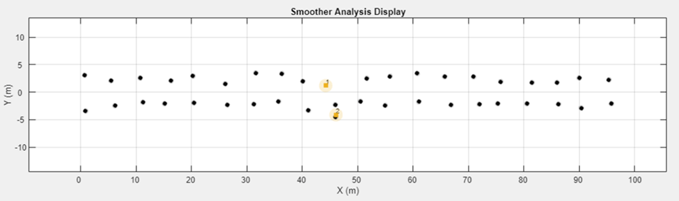
For this scenario, to understand how the smoother associates detections, you pause the simulation at 10 seconds when the data association is ambiguous.

The smoother runs a recursive algorithm from time step 1 to the final time step $N$ , where the first step is the time of the first sensor observation and the last step is the time step of the last sensor observation. In the following subsections, you will learn how the smoother iteration performs from step $k - 1$ to step $k$ .

Forward Predictions

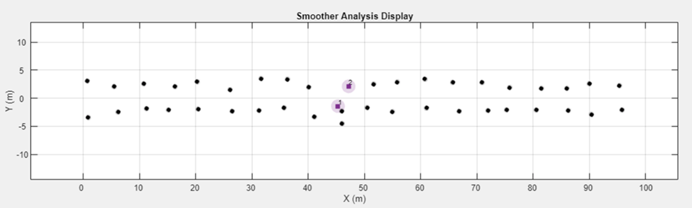
The smoother starts with forward estimates from step $k - 1$ . The forward estimates are estimates of tracks conditional on measurements from step 1 to step $k - 1$ . The first step of the algorithm is forward prediction, where these forward estimates are predicted to step $k$ using a standard Kalman or extended Kalman filter specified by the FilterInitializationFcn property of the smoother. The image below shows the forward predictions at 10 seconds. In the image, there are 2 estimated objects, and their states are predicted using a constant-velocity model. Note that due to noise in the previous measurements, the prediction for track 2 seems closer to the false alarm than its actual measurement.

Backward Predictions

To use future information, the smoother calculates backward predictions. These backward predictions intend to describe the number of objects and their states given measurements from future time instants. In other words, these are predictions about object states at step $k$ , conditional on measurements from step $k + 1$ to step $N$ . The smoother calculates these predictions by running an independent backward-time JIPDA from $N$ to $k + 1$ . The smoother then predicts estimates at step $k + 1$ to step $k$ using the inverse-time dynamics of the motion model described by the filter. Note that the identities of objects calculated by backward JIPDA are independent from the identities in forward predictions. The image below shows the backward predictions at 10 seconds.

Smoothing Predictions

The smoother then proceeds to calculate smoothing predictions. The smoothing predictions describe the number of objects and their states given measurements from past (1 to $k - 1$ ) and future ( $k + 1$ to $N$ ) measurements. The smoother obtains these smoothing predictions by performing a track-to-track assignment between forward predictions and backward predictions using the JIPDA algorithm. The parameters that control the forward-to-backward JIPDA are TrackAssignmentThreshold, TrackAssignmentClassWeight (only applicable for classified tracks) and MaxNumTrackAssignmentEvents properties of the smoother.

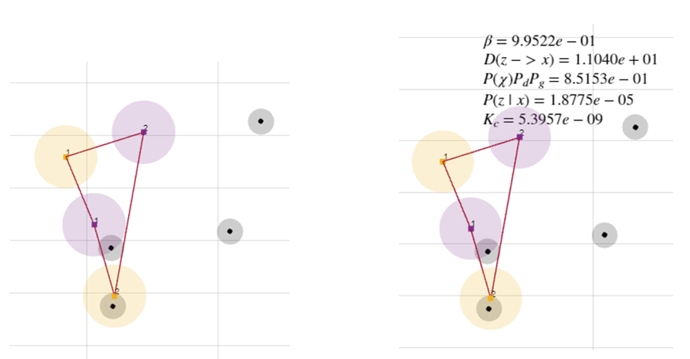
The image below shows the smoothing predictions at 10 seconds. The image on the left shows the data association links considered between forward and backward predictions. You can display these links by selecting the "Data Associations (T2T)" checkbox. The links for data association lines are also interactive. You can click on each link to show more information about the association, as shown on the right. Notice that the estimated association weight between Track 1 from forward prediction and Track 2 from backward prediction is about 0.99522. Additionally, the calculated distance between them is 11.04, the prior probability of assignment (product of forward existence, probability of detection in the future, and probability of finding a backward track inside gate) is 0.85153. The likelihood of association is about 1.8775e-5 and the estimated clutter density is 5.3957e-9.

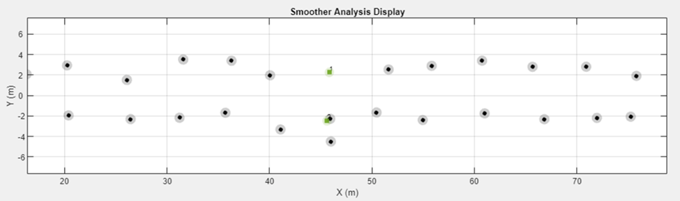
The fusion of forward predictions with backward predictions using probabilistic association results in smoothing predictions. In the image below, you notice the smoothing predictions calculated at the ambiguous time instant. Notice that the smoothing predictions have much smaller uncertainty than forward predictions. Also, the smoothing prediction of track 2 is now much closer to its own detection.

Smoothing Data Associations

At this step, the smoother performs a JIPDA detection-to-track assignment smoothing predictions obtained previously and detections at the current step. The resulting data associations are called smoothing data associations. The parameters that control this detection-to-track assignment are the DetectionAssignmentThreshold, MaxNumDetectionAssignmentEvents, ClutterDensity, DetectionProbability and DetectionAssignmentClassWeight (for classified detections only) properties of the smoother. Similar to track-to-track association, you can also plot the detection-to-track association links calculated by the smoother by selecting the "Data Associations (D2T)" checkbox in the app.

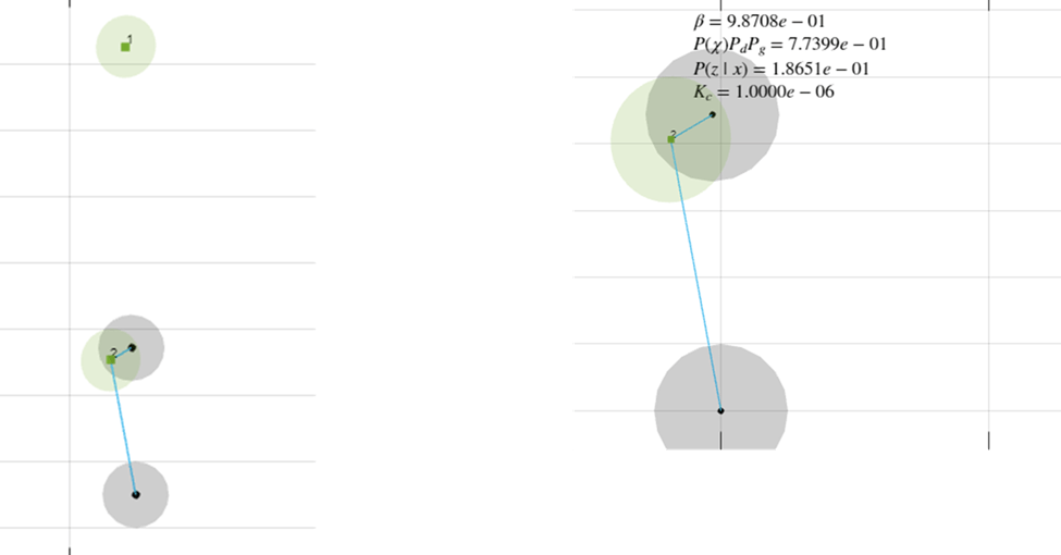
The images below show associations between smoothing predictions and detections at the ambiguous time instant in the scenario. Note that due to much smaller uncertainty of track 1 in the smoothing prediction, the JIPDA process does not consider any association between track 1 and the observed detections. Additionally, track 2 has a strong association weight of 0.98708 with its true detection.

Next, the smoother updates both forward predictions and smoothing predictions with the smoothing data associations to reach step k. You can visualize the updated smooth corrections by selecting the "Smooth Corrections" checkbox.

Once the smoother finishes the iterations from step 1 to step $N$ using the iteration described above, the smoother runs a single-object backward pass (from step $N$ to step 1) on each forward estimate to output the smooth tracks.

% Clear the app and restore the path
close(app.SmootherAnalysisAppUIFigure)
clear app;
if ~appExists
    path(oldPath);
end

Summary

In this example, you learned how the JIPDA smoother computes data association at each step by using future measurements. You also learned how to assess the intermediate results from the smoother using a GUI-based analysis tool. You can use this GUI to assess the performance of the JIPDA smoother and tune its parameters for your own applications.

References

[1] Song, Taek Lyul, and Darko Mušicki. "Smoothing innovations and data association with IPDA." Automatica 48.7 (2012): 1324-1329.

[2] Kim, Tae Han, et al. "Smoothing joint integrated probabilistic data association." IET Radar, Sonar & Navigation 9.1 (2015): 62-66.

[3] Memon, Sufyan, Won Jun Lee, and Taek Lyul Song. "Efficient smoothing for multiple maneuvering targets in heavy clutter." 2016 International Conference on Control, Automation and Information Sciences (ICCAIS). IEEE, 2016.

Supporting Functions

`createSimpleScenarioData`

function [detectionLog, timestamps] = createSimpleScenarioData()
% Random seed for reproducible data
rng(1);

% timestamps
timestamps = 1:20;

% True X Position 
x = 1:5:100; 

% True Y Position
y = 2.5*ones(1,20); 

% True Z Position
z = zeros(1,20);

% Append for both targets
x = [x x];
y = [y -y];
z = [z z];
detectionTimestamps = [timestamps timestamps];

% Add noise
meas = [x;y;z] + 0.5*randn(3,40);

% Missed object at t = 10
meas(:,10) = [];
detectionTimestamps(10) = [];

% False alarm at t = 10
meas(:,end+1) = [x(10);-4.5;0];
detectionTimestamps(end+1) = 10;

% Assemble using objectDetection
detectionLog = cell(size(meas,2),1);
for i = 1:size(meas,2)
    detectionLog{i} = objectDetection(detectionTimestamps(i),meas(:,i),'MeasurementNoise',0.25*eye(3));
end

end