Surrogate Optimization with Nonlinear Constraint
This example shows how to include nonlinear inequality constraints in a surrogate optimization. The example solves an ODE with a nonlinear constraint. The example Optimize ODEs in Parallel shows how to solve the same problem using other solvers that accept nonlinear constraints.
For a video overview of this example, see Surrogate Optimization.
Problem Description
The problem is to change the position and angle of a cannon to fire a projectile as far as possible beyond a wall. The cannon has a muzzle velocity of 300 m/s. The wall is 20 m high. If the cannon is too close to the wall, it fires at too steep an angle, and the projectile does not travel far enough. If the cannon is too far from the wall, the projectile does not travel far enough.
Nonlinear air resistance slows the projectile. The resisting force is proportional to the square of velocity, with the proportionality constant 0.02. Gravity acts on the projectile, accelerating it downward with constant 9.81 m/s^2. Therefore, the equations of motion for the trajectory x(t) are
where .
The initial position x0 and initial velocity xp0 are 2-D vectors. However, the initial height x0(2) is 0, so the initial position is given by the scalar x0(1). The initial velocity has magnitude 300 (the muzzle velocity) and, therefore, depends only on the initial angle, which is a scalar. For an initial angle th, the initial velocity is xp0 = 300*(cos(th),sin(th)). Therefore, the optimization problem depends only on two scalars, making it a 2-D problem. Use the horizontal distance and initial angle as the decision variables.
Formulate ODE Model
ODE solvers require you to formulate your model as a first-order system. Augment the trajectory vector with its time derivative to form a 4-D trajectory vector. In terms of this augmented vector, the differential equation becomes
The cannonshot file implements this differential equation.
function f = cannonshot(~,x)
    f = [x(3);x(4);x(3);x(4)]; % initial, gets f(1) and f(2) correct
    nrm = norm(x(3:4)) * .02; % norm of the velocity times constant
    f(3) = -x(3)*nrm; % horizontal acceleration
    f(4) = -x(4)*nrm - 9.81; % vertical acceleration
end
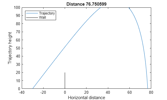
Visualize the solution of this ODE starting 30 m from the wall with an initial angle of pi/3. The plotcannonsolution function uses ode45 to solve the differential equation.
function dist = plotcannonsolution(x)
    % Change initial 2-D point x to 4-D x0
    x0 = [x(1);0;300*cos(x(2));300*sin(x(2))];
    sol = ode45(@cannonshot,[0,15],x0);
    % Find the time when the projectile lands
    zerofnd = fzero(@(r)deval(sol,r,2),[sol.x(2),sol.x(end)]);
    t = linspace(0,zerofnd); % equal times for plot
    xs = deval(sol,t,1); % interpolated x values
    ys = deval(sol,t,2); % interpolated y values
    plot(xs,ys)
    hold on
    plot([0,0],[0,20],"k") % Draw the wall
    xlabel("Horizontal distance")
    ylabel("Trajectory height")
    ylim([0 100])
    legend("Trajectory","Wall",Location="NW")
    dist = xs(end);
    title(sprintf("Distance %f",dist))
    hold off
end
plotcannonsolution uses fzero to find the time when the projectile lands, meaning its height is 0. The projectile lands before time 15 s, so plotcannonsolution uses 15 as the amount of time for the ODE solution.
x0 = [-30;pi/3];
dist = plotcannonsolution(x0);
Prepare Optimization
To optimize the initial position and angle, write a function similar to the previous plotting routine. Calculate the trajectory starting from an arbitrary horizontal position and initial angle.
Include sensible bound constraints. The horizontal position cannot be greater than 0. Set an upper bound of –1. Similarly, the horizontal position cannot be below –200, so set a lower bound of –200. The initial angle must be positive, so set its lower bound to 0.05. The initial angle should not exceed pi/2; set its upper bound to pi/2 – 0.05.
lb = [-200;0.05];
ub = [-1;pi/2-.05];
Write an objective function that returns the negative of the resulting distance from the wall, given an initial position and angle. If the trajectory crosses the wall at a height less than 20, the trajectory is infeasible; this constraint is a nonlinear constraint. The cannonobjcon function implements the objective function calculation. To implement the nonlinear constraint, the function calls fzero to find the time when the x-value of the projectile is zero. The function accounts for the possibility of failure in the fzero function by checking whether, after time 15, the x-value of the projectile is greater than zero. If not, then the function skips the step of finding the time when the projectile passes the wall.
function f = cannonobjcon(x)
    % Change initial 2-D point x to 4-D x0
    x0 = [x(1);0;300*cos(x(2));300*sin(x(2))];
    % Solve for trajectory
    sol = ode45(@cannonshot,[0,15],x0);
    % Find time t when trajectory height = 0
    zerofnd = fzero(@(r)deval(sol,r,2),[1e-2,15]);
    % Find the horizontal position at that time
    dist = deval(sol,zerofnd,1);
    % What is the height when the projectile crosses the wall at x = 0?
    if deval(sol,15,1) > 0
        wallfnd = fzero(@(r)deval(sol,r,1),[0,15]);
        height = deval(sol,wallfnd,2);
    else
        height = deval(sol,15,2);
    end
    f.Ineq = 20 - height; % height must be above 20
    % Take negative of distance for maximization
    f.Fval = -dist;
end
You already calculated one feasible initial trajectory. Use that value as an initial point.
fx0 = cannonobjcon(x0);
fx0.X = x0;
Solve Optimization Using surrogateopt
Set surrogateopt options to use the initial point. For reproducibility, set the random number generator to default. Use the "surrogateoptplot" plot function. Run the optimization. To understand the "surrogateoptplot" plot, see Interpret surrogateoptplot.
opts = optimoptions("surrogateopt",InitialPoints=x0,PlotFcn="surrogateoptplot");
rng default
[xsolution,distance,exitflag,output] = surrogateopt(@cannonobjcon,lb,ub,opts)
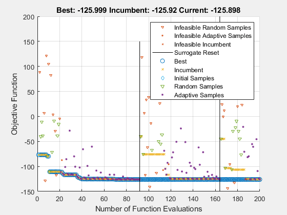
surrogateopt stopped because it exceeded the function evaluation limit set by
'options.MaxFunctionEvaluations'.
xsolution = 1×2

  -28.4081    0.6160
distance =
-125.9988
exitflag =
0
output = struct with fields:
        elapsedtime: 18.7102
          funccount: 200
    constrviolation: 8.4347e-04
               ineq: 8.4347e-04
           rngstate: [1×1 struct]
            message: 'surrogateopt stopped because it exceeded the function evaluation limit set by ↵'options.MaxFunctionEvaluations'.'
Plot the final trajectory.
figure
dist = plotcannonsolution(xsolution);
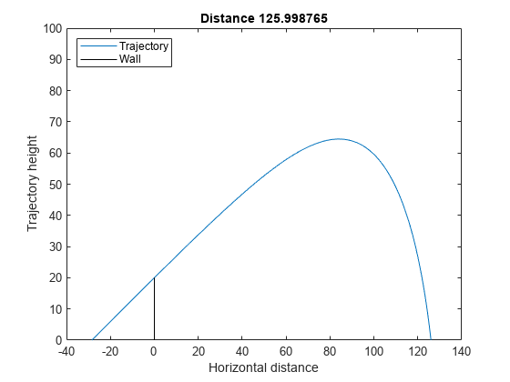
The patternsearch solution in Optimize ODEs in Parallel shows a final distance of 125.9880, which is almost the same as this surrogateopt solution.