HDL Code Generation for Streaming Matrix Inverse System Object
This example shows how HDL Coder™ implements a streaming mode of matrix inverse operation with configurable sizes.
What is inverse of a matrix
A matrix X is invertible if there exists a matrix Y of the same size such that XY = YX = I, where I is the Identity matrix. The matrix Y is called inverse of X. A matrix that has no inverse is singular. A square matrix is singular only when its determinant is exactly zero.
Matrix inverse computation involves following steps:
Cofactor matrix calculation
Transpose of cofactor matrix
Multiply reciprocal of determinant of input matrix with transpose of cofactor matrix
Example:
             A = [4 12 -16;12 37 -43;-16 -43 98];
Cofactors of 'A' will be calculated from matrix of minors
        cof(A) = [1777 488 76;488 136 20;76 20 4];
Transpose of cofactor matrix will be
(cof(A))' = [1777 488 76;488 136 20;76 20 4];Multiply reciprocal of determinant of 'A' with transpose of cofactor matrix
Ainv = (1/det(A)) * (cof(A))'
= [49.3611 -13.5556 2.1111;-13.5556 3.7778 -0.5556;2.1111 -0.5556 0.1111];Matrix Inverse: Gauss-Jordan elimination
To find the inverse of matrix A using Gauss-Jordan elimination, we must find elementary row operations that reduce A to identity matrix(I) and then perform the same operations on Identity matrix(I) to obtain Ainv.
Computation of Matrix Inverse using Gauss-Jordan elimination: Let start with matrix A, and write it down with an Identity matrix next to it: [A | I]
The goal is to make A an identity matrix by applying row transformations and right-hand side matrix I also participated in the row transformations, finally reduced to Ainv.
Computation of Ainv involves following steps:
swapping rows
make the diagonal elements as 1
make the non-diagonal elements as 0
Example:
                    (A)       (I)
                  1  2  3 | 1  0  0
      [A | I] =   2  5  3 | 0  1  0
                  1  0  8 | 0  0  1
Find the element with maximum value in the first column and swap the current
row with maximum element row
swap R1 and R2 rows as R2 contains the largest values. 2 5 3 | 0 1 0
= 1 2 3 | 1 0 0
1 0 8 | 0 0 1Make the diagonal element in the first column as '1'
R1 --> R1/2 1 2.5 1.5 | 0 0.5 0
= 1 2 3 | 1 0 0
1 0 8 | 0 0 1
Make the non-diagonal elements in the first column as '0'
R2 --> R2 - R1
R3 --> R3 - R1 1 2.5 1.5 | 0 0.5 0
= 0 -0.5 1.5 | 1 -0.5 0
0 -2.5 6.5 | 0 -0.5 1Now column 1 has diagonal elements '1' and other elements as '0'. This procedure is repeated for remaining columns and matrix A will be reduced to identity matrix, Identity matrix will be reduced to Ainv.
                  1  0  0 | -40  16   9
              =   0  1  0 |  13  -5  -3
                  0  0  1 |   5  -2  -1
                    (I)        (Ainv)
Matrix Inverse: Cholesky decomposition
Matrix Inverse using cholesky decomposition supports only symmetric positive definite matrices. Positive definite means all the eigenvalues of the matrix should be positive.
Given a symmetric positive definite matrix A:
           A   = L * L',             L  is the lower triangular matrix
                                     L' is the transpose of L
inv(A) = inv(L * L')
= inv(L') * inv(L)
= (inv(L))' * inv(L) Ainv = Linv' * Linv, Linv is the inverse of lower triangular matrix
Ainv is the inverse of input matrixComputation of Ainv involves following steps:
Lower triangular matrix computation(L)
Inverse of lower triangular matrix(Linv)
Multiplication of transpose of Linv with Linv
Example:
A = [4 12 -16;12 37 -43;-16 -43 98];
Lower triangular matrix(L) will be computed using cholesky decomposition
             L = [2 0 0;6 1 0;-8 5 3];
Linv will be computed using forward substitution method
Linv = [0.5 0 0;-3 1 0;6.3333 -1.6667 0.3333];Multiply transpose of Linv with Linv
Ainv = Linv' * Linv
= [49.3611 -13.5556 2.1111;-13.5556 3.7778 -0.5556;2.1111 -0.5556 0.1111];Benefits of using Gauss-Jordan Elimination
Gauss-Jordan Elimination supports all square matrices.
Gauss-Jordan Elimination supports both
singleanddoubledata types.
Restrictions for Cholesky implementation
Matrices for which inverse is to computed must be symmetric positive-definite.
Input data types of the matrices must be
singleand block must be used in theNative Floating Pointmode.Input matrices must not be larger than 64-by-64 in size.
Matrix Inverse Subsystem Interface:
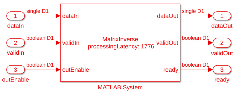
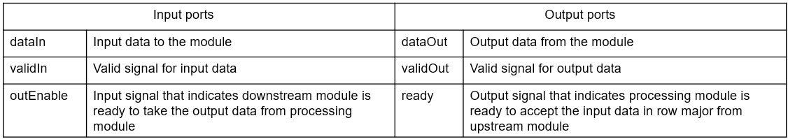
Matrix Inverse ports description:
Matrix Inverse Implementation
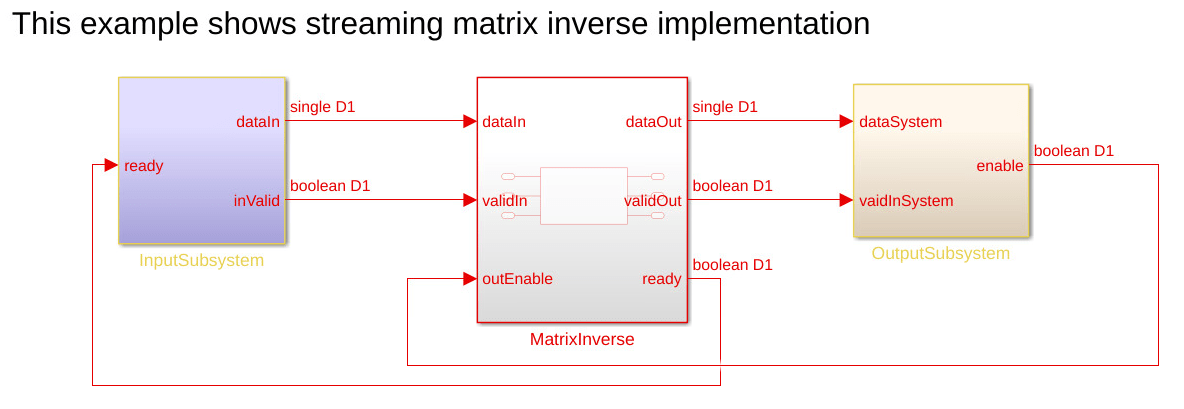
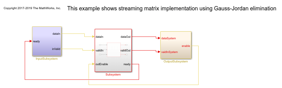
This example model contains three subsystems: InputSubsystem, MatrixInverse, and OutputSubsystem. The InputSubsystem is the upstream module that serializes the matrix input to the processing module when the ready signal is enabled. The OutputSubsystem is the downstream module that deserializes the data from the processing module to a matrix output when the outEnable signal is enabled. The MatrixInverse is a processing module that implements the matrix inverse operation.
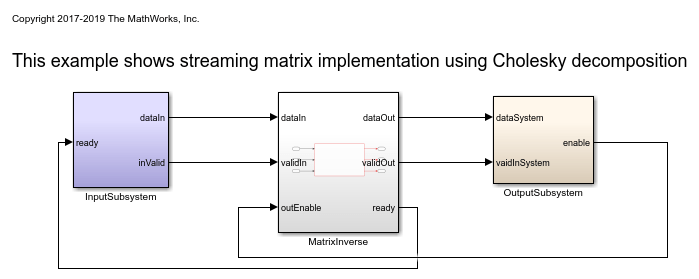
open_system('hdlcoder_streaming_mat_inv_max_lat_cholesky');
open_system('hdlcoder_streaming_mat_inv_max_lat_gauss_jordan');
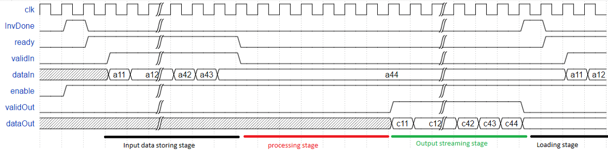
Matrix Inverse Timing diagrams:
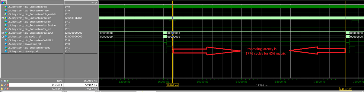
Timing diagram for complete system:
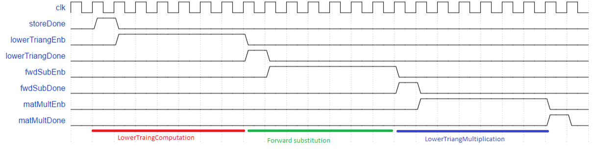
Timing diagram for processing stage(Cholesky decomposition):
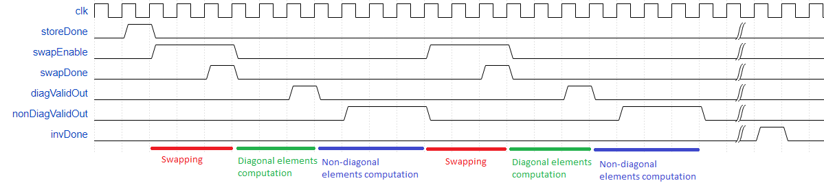
Timing diagram for processing stage(Gauss-Jordan elimination):
Modelsim result waveform(Cholesky decomposition)
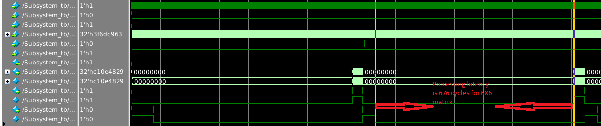
Modelsim result waveform(Gauss-Jordan elimination)
Matrix Inverse Block parameters:
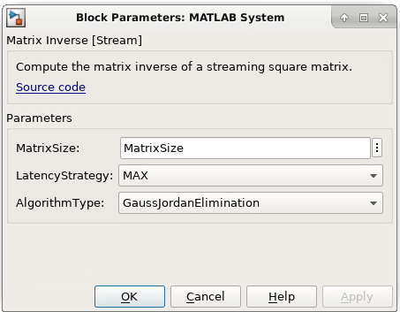
MatrixSize : Enter size of input matrix as a positive integer.
LatencyStrategy : Select latency strategy from drop down menu
                   ({'ZERO, 'MIN', 'MAX'}) which should be same as HDL coder
                   latency strategy. User can see processing latency
                   based on the latency strategy.
AlgorithmType   : Select algorithm type from drop down menu({'CholeskyDecomposition',
                   'GaussJordanElimination'})
Matrix Inverse Block usage
Set block parameters of MATLAB System block.
Select input matrix based on the matrix size.
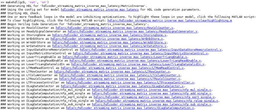
Generate HDL code for MatrixInverse subsystem.
Generated code and Generated model
After running code generation for MatrixInverse subsystem, generated code will be
Generated model contains the MatrixInverse MATLAB System block. During modelsim simulation code generation outputs are compared with MATLAB System block outputs.
Synthesis statistics
Cholesky decomposition
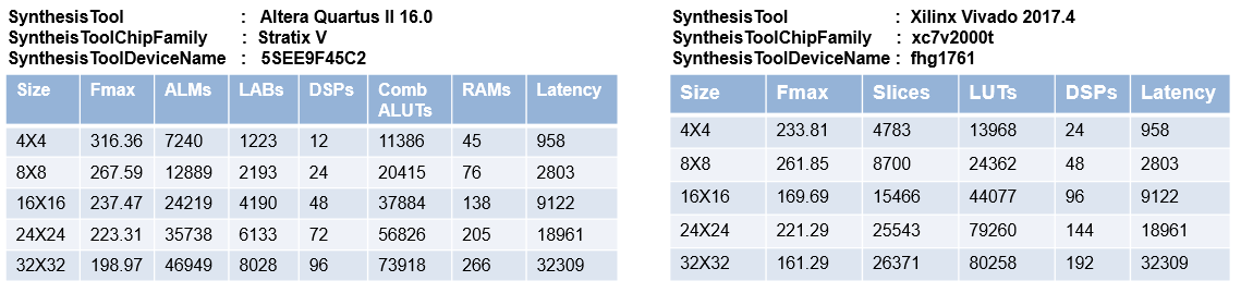
Gauss-Jordan elimination
