Cylinder Design Parameter Estimation
This example shows how to parameterize and test a tandem primary cylinder starting from a manufacturer datasheet. This example uses optimization to determine remaining unknown parameters, given the numerical data extracted from the datasheet. After the model is simulated, it compares the resulting push rod force - brake pressure relationship curve to the curve provided on the manufacturer datasheet. Understanding the behavior of the tandem primary cylinder is important when selecting other braking system components.
The live script requires the Optimization Toolbox™ and Global Optimization Toolbox to be installed and licensed to run.
Model
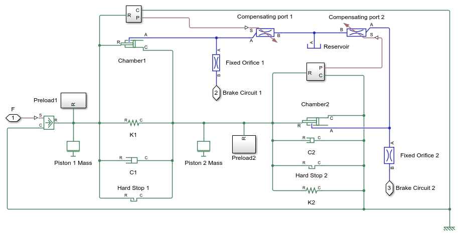
The following figure shows the tandem primary cylinder test harness. The model uses spring-loaded accumulators for loading in the  and the
  circuits in place of disk or drum brakes. The input to the model is the push rod force coming from the lever mechanism or the brake booster. The output of the model is the pressures achieved in the brake circuits 1 and 2 respectively.

Manufacturer Datasheet Data
The supplier has provided the following data in the datasheet.
tpcPistonDiameter : first and second circuit piston diameter.
tpcPistonStroke1 : first circuit piston stroke.
tpcPistonStroke2 : second circuit piston stroke.
tpcTotalStroke : overall stroke.
tpcCircuit1Disp : first circuit displacement.
tpcCircuit2Disp : second circuit displacement.
tpcTotalDisp : net displacement.
_tpcMaxPressure _ : max pressure.
Pressure Development Characteristics
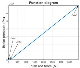
The supplier datasheet gives the following function diagram for the push rod force-brake pressure curve for the tandem primary cylinder which should be followed by the brake circuit 1 and 2 as per supplier catalog. It is required for a tandem primary cylinder to have same brake pressures created in brake circuits for uniform braking.

Equations of Motion (EoM) of System
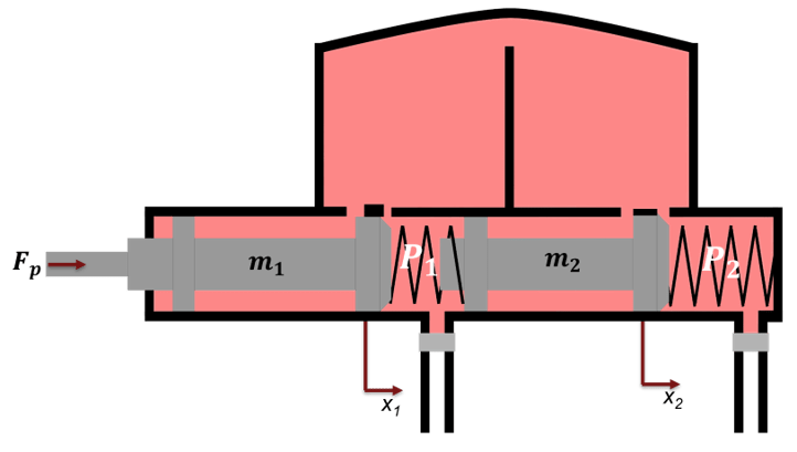
The following figure shows the tandem primary cylinder. Mass 1 and mass 2 use the coordinate frames shown below. This description only includes the mechanical EoM of the system. The fluid dynamics equations are not shown.
 , when
 , when
 , when
 , when
where,
 and
and  are positions of piston mass 1 and mass 2 from the left side assumed hard stop.
 and
and  are masses of piston 1 and 2 respectively.
 and
and  are damping coefficients of piston 1 and 2 respectively.
 and
and  are stiffness coefficients of left (Spring 1) and right (spring 2) respectively.
 is force applied on push rod of primary cylinder.
 and
and  are pressures in brake circuit 1 and 2 respectively.
 and
and  are reaction forces on mass 1 and 2 respectively when both masses are at the leftmost position.
 and
and  are preloads on left and right side springs respectively.
Parameter Estimation Scheme
The following steps outline how to estimate unknown feasible parameters of the tandem primary cylinder.
1. Identify Parameters to be Estimated
Some parameters, which are required for component model simulation, are not provided in the manufacturer's datasheet. Therefore, in order to validate the model with supplier function diagram it is necessary to estimate these parameters. The supplier function diagram gives quasi- steady state behavior of the tandem primary cylinder.
Where,
Data1, Data2, and Data3 are 3 points on the manufacturer function diagram.
Data1 point represents the leftmost points of the pistons in their respective coordinate frames.
Data3 point represent the right most points of the pistons in their respective coordinate frame, which are given in the datasheet.
Data2 point represent pistons movement at which brake circuits 1 and 2 get disconnected from the brake oil reservoir by the closing of the compensating ports. Movement beyond Data2 point in the right direction results in pressure building in the brake circuits. These points are not given in the datasheet and have to be estimated.
Left and right spring stiffness coefficients and pre-compressions are unknown.
Therefore there are 6 unknown parameters.
tpcPosOpen1, which is piston 1 movement up to which compensating port remains connected with the brake circuit 1.
tpcPosOpen2, which is piston 2 movement up to which compensating port remains connected with the brake circuit 2.
tpcStiffness1Coeff, which is first spring stiffness coefficient
tpcStiffness2Coeff, which is second spring stiffness coefficient
tpcSpring1Comp, which is first spring pre-compression displacement
tpcSpring2Comp, which is second spring pre-compression displacement. This parameter can be computed from the constraint that the Preload1 and Preload2 are equal at rest in the steady state of the system.
The datasheet does not provide the step test data, therefore the overshoot, rise time, settling time, and recovery time are not known. Therefore, the inertia and damping coefficient can't be estimated.
2. Provide Lower, Upper Bound, Scaling Factor and Initialization Point for the Parameter Estimation through Optimization
Defining scaling factor for better numerical performance of the optimization algorithm
Defining lower bound vector for optimization
Defining upper bound vector for optimization
Computing initialization point between lower and upper bound for the optimization algorithm for parameter estimation.
Defining random initialization point for the optimization
3. Define Objective Function
The optimization algorithm minimizes the objective function to estimate the required unknown parameters. The function used here defines the least squared error between the simulation output and the expected output from the datasheet. The Error Objective subsystem computes the least squared error vector.

Open objective function definition file to see the cumulative error estimation code.
The optimization algorithm assumes that the objective function has one input x, where x has as many elements as the number of unknown variables in the problem. The objective function computes the scalar value of the objective function and returns it in its single output argument y.
4. Setting up model for Fast Restart
You can save computational time by setting up the model in Fast Restart mode. Set parameter configurability to Run-Time so that optimization algorithm can be executed in Fast Restart mode. This requires modeling spring pre-compressions and preload through Ideal force Source blocks in the model.
5. Parameter Estimation Using Optimization Algorithm
It is important to choose an algorithm which matches the problem complexity and type. No single optimization algorithm can perform the same for all types of problems.
Defining objective function
Defining lower bound
Defining upper bound
Defining optimization initialization point
You can use a hybrid algorithm to estimate unknown parameters. In a hybrid algorithm, multiple algorithms are re used together. For example, first a Global optimization algorithm, such as Simulated Annealing, could perform the optimization iterations, and then feed the output to a gradient based optimization algorithm such as fmincon to refine the optimization output.
You can also use other existing optimization algorithm functions such as Pattern Search, lsqnonlin, Genetic Algorithm, or Particle Swarm. However, you need to reconfigure optimization options for better results.
You can use Surrogate optimization to estimate the unknown parameters. Here optimization is performed using Surrogate optimization.
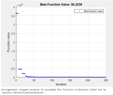
The estimated parameters are converted to their respective values through the defined scale.
Converting scaled parameters to actual values.
Switching off Fast Restart
Simulation
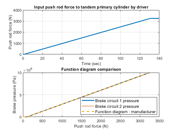
The model generates push rod force-brake pressure plots for the selected manufacturer design based on the optimization algorithm parameter estimation. The applied push rod force to the tandem primary cylinder is ramped at 25 N/sec rate in the simulation.
Plotting output from Simscape™ tandem primary cylinder model and comparing with function diagram