Estimate Soil Moisture Using Temperature Vegetation Dryness Index

R2026b

Since R2026b

This example shows how to estimate relative soil moisture from Landsat 8 multispectral satellite imagery by computing the temperature vegetation dryness index (TVDI).

Monitoring soil moisture is critical for precision agriculture, drought assessment, and land management. Satellite-based approaches enable large-scale estimation without ground instrumentation. The TVDI leverages the relationship between land surface temperature (LST) and the normalized difference vegetation index (NDVI) to characterize surface moisture conditions [1].

When LST is plotted against NDVI for a scene, the data typically forms a triangular distribution. The lower boundary of this triangle represents the minimum LST at each NDVI value and corresponds to well-watered surfaces (the wet edge). The upper boundary represents the maximum LST and corresponds to moisture-limited surfaces (the dry edge). TVDI quantifies where each pixel falls between these two edges, producing a value between 0 (wet) and 1 (dry).

In this example, you perform these steps:

1. Load and preprocess Landsat 8 multispectral data.

2. Compute land surface temperature (LST) from the thermal band.

3. Compute the Normalized Difference Vegetation Index (NDVI).

4. Derive the LST-NDVI triangular relationship.

5. Calculate the TVDI for the scene.

6. Visualize the soil moisture estimation results.

This example requires the Hyperspectral Imaging Library for Image Processing Toolbox™. You can install the Hyperspectral Imaging Library for Image Processing Toolbox from Add-On Explorer. For more information about installing add-ons, see Get and Manage Add-Ons.

Load and Preprocess Multispectral Data

Landsat 8 is an Earth observation satellite that carries the Operational Land Imager (OLI) and Thermal Infrared Sensor (TIRS) instruments. The Landsat 8 data set has 11 spectral bands with wavelengths that range from 440 nm (coastal aerosol) to 12510 nm (thermal infrared).

Download the data set and unzip the file by using the downloadLandsat8Dataset helper function. The helper function is attached to this example as a supporting file.

zipfile = "LC08_L1TP_197049_20231122_20231122_02_RT.zip";
landsat8Data_url = "https://ssd.mathworks.com/supportfiles/image/data/" + zipfile;
downloadLandsat8Dataset(landsat8Data_url,pwd)

Read the Landsat 8 multispectral data into the workspace using the immulticube function.

filepath = fullfile("LC08_L1TP_197049_20231122_20231122_02_RT","LC08_L1TP_197049_20231122_20231122_02_RT_MTL.txt");
mcube = immulticube(filepath);

Resample the bands to a uniform spatial resolution of 30 meters per pixel. Landsat 8 acquires different bands at different resolutions, so resampling ensures consistent pixel alignment across bands.

mcube = resampleBands(mcube,30);

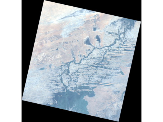
Generate an RGB rendering of the scene for visual reference.

rgbImg = colorize(mcube);
figure
imageshow(rgbImg)

Compute Land Surface Temperature

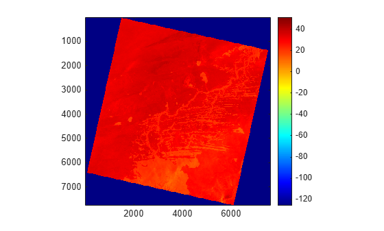
Land surface temperature (LST) represents the radiative temperature of the ground surface. For simplicity, this example uses brightness temperature as a proxy for LST, omitting emissivity correction. To compute LST from Landsat 8 data, convert the raw digital numbers in the thermal infrared band (band 10) to spectral radiance, then convert radiance to brightness temperature.

Select the thermal infrared band (band 10) from the multicube and gather the data into a numeric array.

mcubeThermal = selectBands(mcube,BandNumber=10);
thermal = gather(mcubeThermal);

Define the radiometric calibration constants from the metadata file LC08_L1TP_197049_20231122_20231122_02_RT_MTL.txt. The radiometric calibration constants are listed in the file under the group title GROUP = LEVEL1_RADIOMETRIC_RESCALING.

Identify the radiance multiplicative rescaling factor for band 10 from the RADIANCE_MULT_BAND_10 value in the file and assign it to the variable ML.

ML = 0.0003342;

Identify the radiance additive rescaling factor for band 10 from the RADIANCE_ADD_BAND_10 value in the file and assign it to the variable AL.

AL = 0.1;

Define the thermal conversion constants from the metadata file LC08_L1TP_197049_20231122_20231122_02_RT_MTL.txt. The thermal conversion constants are listed in the file under the group title GROUP = LEVEL1_THERMAL_CONSTANTS.

Identify the K1 constant for band 10 from the K1_CONSTANT_BAND_10 value in the file and assign it to the variable K1.

K1 = 774.8853;

Identify the K2 constant for band 10 from the K2_CONSTANT_BAND_10 value in the file and assign it to the variable K2.

K2 = 1321.0789;

Convert the digital numbers to top-of-atmosphere spectral radiance using the multiplicative and additive rescaling factors.

radiance = ML*double(thermal)+AL;

Convert radiance to brightness temperature in Kelvin using the Planck-derived inversion formula, then convert to degrees Celsius.

lst = K2./log(K1./radiance+1);
lstImg = lst-273.15;

Display the LST map.

figure
imagesc(lstImg)
axis equal tight
colormap(jet)
colorbar

Compute the Normalized Difference Vegetation Index

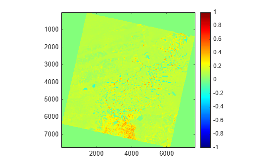
NDVI quantifies vegetation density and health using the contrast between near-infrared (NIR) and red reflectance. Dense, healthy vegetation reflects strongly in the NIR and absorbs in the red, producing high NDVI values. Bare soil and urban areas produce values near zero.

Compute NDVI directly from the multicube using the ndvi function.

ndviImg = ndvi(mcube);

Display the NDVI map.

figure
imagesc(ndviImg)
axis equal tight
colormap(jet)
colorbar

Derive the LST-NDVI Triangular Relationship

The triangular space formed by plotting LST against NDVI defines the wet and dry edges needed to compute TVDI. To extract these edges, bin the NDVI values into intervals and determine the minimum and maximum LST within each bin.

Flatten the NDVI and LST arrays for statistical analysis.

ndviFlat = ndviImg(:);
lstFlat = lstImg(:);

Divide the NDVI range into 20 equally spaced bins and compute the 5th percentile (wet edge) and 95th percentile (dry edge) of LST within each bin.

numBins = 20;
edges = linspace(min(ndviFlat),max(ndviFlat),numBins+1);
ndviBinCenters = zeros(numBins,1);
lstMin = zeros(numBins,1);
lstMax = zeros(numBins,1);

for i = 1:numBins
    binIdx = ndviFlat>=edges(i) & ndviFlat<edges(i+1);
    binLST = lstFlat(binIdx);
    if ~isempty(binLST)
        ndviBinCenters(i) = mean(edges(i:i+1));
        lstMin(i) = prctile(binLST,5);
        lstMax(i) = prctile(binLST,95);
    else
        ndviBinCenters(i) = NaN;
        lstMin(i) = NaN;
        lstMax(i) = NaN;
    end
end

Fit linear models to the wet edge and dry edge across the NDVI bins. The wet edge is defined as $$LS{T}_{min}=a\cdot NDVI+b$$ and the dry edge as $$LS{T}_{max}=c\cdot NDVI+d$$.

valid = ~isnan(ndviBinCenters);
pMin = polyfit(ndviBinCenters(valid),lstMin(valid),1);
pMax = polyfit(ndviBinCenters(valid),lstMax(valid),1);

Calculate the TVDI

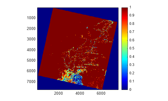
Compute the TVDI for each pixel using the linear models of the wet and dry edges. The index represents the relative position of each pixel between the wet edge (TVDI = 0, indicating moist surface conditions) and the dry edge (TVDI = 1, indicating dry surface conditions) [1]:

$$TVDI=\frac{LST-LS{T}_{min}(NDVI)}{LS{T}_{max}(NDVI)-LS{T}_{min}(NDVI)}$$

Predict the wet edge and dry edge LST values for each pixel based on its NDVI value.

lstMinMap = polyval(pMin,ndviImg);
lstMaxMap = polyval(pMax,ndviImg);

Compute the TVDI and clamp the values to the range [0, 1].

tvdi = (lstImg-lstMinMap)./(lstMaxMap-lstMinMap);
tvdiImg = min(max(tvdi,0),1);

Display the TVDI map.

figure
imagesc(tvdiImg)
axis equal tight
colormap(jet)
colorbar

References

[1] Sandholt, I., K. Rasmussen, and J. Andersen. "A Simple Interpretation of the Surface Temperature/Vegetation Index Space for Assessment of Surface Moisture Status." Remote Sensing of Environment 79, no. 2–3 (2002): 213–224. https://doi.org/10.1016/S0034-4257(01)00274-7.