Export Figures for Use in Other Applications

Since R2025a. Replaces Save Figure with Specific Size, Resolution, and Background Color (R2024b) and Saving and Copying Plots with Minimal White Space (R2024b).

To export figures and plots for use in documents and other applications, use the exportgraphics function to save your content in a file, or use the copygraphics function to copy your content to the clipboard. Both functions enable you to capture figures and plots with the appropriate size, resolution, and aspect ratio for your application. You can also specify a margin of padding, a background color, and control axes tick placement. The examples in this topic use the exportgraphics function, but you can apply the same concepts and arguments when using the copygraphics function.

When you use the exportgraphics and copygraphics functions, UI components and containers, such as panels, that are next to your plot are excluded from the saved content. For these cases, use the exportapp function instead.

Specify Graphics to Export

To export a plot to a file, use the exportgraphics function. Specify the parent figure as the first argument. For example, create a figure that is 535-by-325 pixels in size. Then create a contour plot and export the figure as a PNG file. Specifying the figure enables you to capture all axes objects directly parented to the figure and their contents. If your figure contains annotations, exportgraphics captures the annotations as well.

f = figure;
f.Position(3:4) = [535 325];
contour(peaks)
colorbar
exportgraphics(f,"contour.png")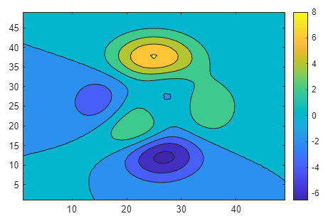

Alternatively, you can specify an axes object instead of a figure as the first argument to the exportgraphics function. In this case, the resulting file is the same because the figure contains only one axes object.

ax = gca;
exportgraphics(ax,"contour.png")

You can also export a tiling of plots by passing a TiledChartLayout object as the first argument. For example, create a tiling of two plots and export the tiled chart layout as a PNG file.

f = figure;
f.Position(3:4) = [650 300];
t = tiledlayout(1,2);
ax1 = nexttile;
plot([4 3 2; 3 2 1],LineWidth=2)
ax2 = nexttile;
contourf(peaks)
exportgraphics(t,"twoplots.png")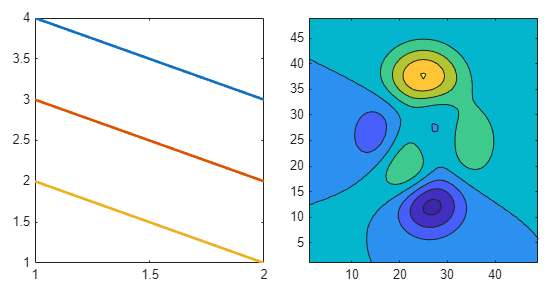

To export one plot from a tiled chart layout, use the nexttile function to get the axes object and pass it to the exportgraphics function. For example, nexttile(2) returns the axes in the second tile.

ax = nexttile(2);
exportgraphics(ax,"secondplot.png")

Specify Resolution

To export a plot as an image at a specific resolution, use the exportgraphics function with the Resolution name-value argument. By default, images are saved at 150 dots per inch (DPI).

A common resolution for printed output is 300 DPI. For graphics on the web, a typical resolution is 72 DPI. To export a plot using the same resolution as MATLAB^® uses, use the value of the ScreenPixelsPerInch property of the graphics root (groot) object. Regardless of the resolution you specify, the pixel dimensions of the final image are approximately the width and height of the figure multiplied by the resolution. For instance, exporting a 4-inch-wide plot at 300-DPI results in a 1200-pixel-wide image.

For example, create a figure that is 535-by-325 pixels in size. Then create a bar chart and export the chart using the same resolution as MATLAB uses.

f = figure;
f.Position(3:4) = [535 325];
bar([1 11 7 8 2 2 9 3 6])
sppi = get(groot,"ScreenPixelsPerInch");
exportgraphics(f,"barchart.png",Resolution=sppi)

You can export plots of a specific size by specifying the resolution as well as the width and height. For example, this code saves the contents of a figure as a 300-DPI, 3-inch square (or 900-pixels square) image. More details on specifying the width and the height are provided in the following sections.

exportgraphics(gcf,"bar-3inch-300dpi.png",Units="inches", ...
       Width=3,Height=3,Resolution=300)

Specify Size

The exportgraphics function has four name-value arguments that enable you to control the dimensions and aspect ratio when exporting a plot: Width, Height, Units, and PreserveAspectRatio.

A simple way to control the size of the output file is to specify the length of one dimension using either the Width or the Height name-value argument. MATLAB adjusts the dimension you do not specify to preserve the original aspect ratio. Specify the Units name-value argument when you specify the Width or Height values.

When you specify the size, also adjust the Position property of the figure so that the width and height of the figure are similar to the desired width and height of the exported file. The Position property is a four-element vector. The width and height values are the last two elements of the vector (in pixel units by default). Make this adjustment before calling exportgraphics.

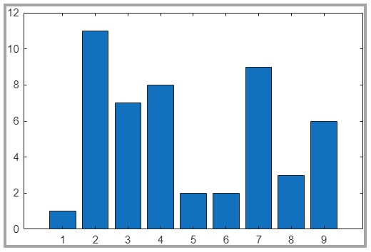
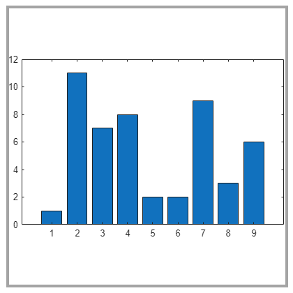
For example, create a figure that is 535-by-325 pixels in size. Create a bar chart and save it as a PNG file that is approximately 500 pixels wide. MATLAB adjusts the height to be 334 pixels to maintain the original aspect ratio. By default, the content is tightly cropped around the axes. The gray border around the image outlines the captured region. The border is not part of the saved image.

f = figure;
f.Position(3:4) = [535 325];
bar([1 11 7 8 2 2 9 3 6])
exportgraphics(f,"bar500.png",Units="pixels",Width=500)

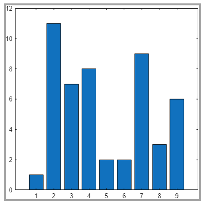
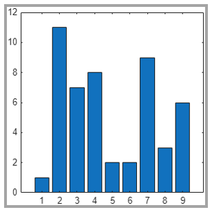
You can also specify both the Width and the Height values. This code changes the aspect ratio to create a tightly cropped, square image.

exportgraphics(f,"barsquare.png", ...
        Units="pixels",Width=400,Height=400)

If you want to preserve the original aspect ratio of the chart, specify the PreserveAspectRatio name-value argument as "on". This code creates a square image that includes padding to preserve the original aspect ratio of the bar chart.

exportgraphics(f,"barsquare-padded.png", ...
        Units="pixels",Width=400,Height=400,PreserveAspectRatio="on")

If you export an image file and specify the width or height using nonpixel units, such as inches or centimeters, be sure to specify the Resolution name-value argument. Otherwise, the output has a default resolution of 150 DPI, which might result in a different size than is required for your application.

For example, create a bar chart and save it as a 3-inch-square image using the same resolution as MATLAB uses.

f = figure;
f.Position(3:4) = [300 300];
bar([1 11 7 8 2 2 9 3 6])
sppi = get(groot,"ScreenPixelsPerInch");
exportgraphics(f,"bar3inchsquare.png", ...
        Units="inches",Width=3,Height=3, ...
        Resolution=sppi)

An alternative way to control the size is to save the content as a vector graphics file. Then you can resize the content in your final application. To save the content as a vector graphics file, use the exportgraphics function with the ContentType name-value argument specified as "vector". For example, create a bar chart and save the figure as an PDF fragment containing vector graphics. All fonts are included in the PDF file. The output file looks similar to this image.

f = figure;
f.Position(3:4) = [535 325];
bar([1 11 7 8 2 2 9 3 6])
exportgraphics(f,"bar.pdf",ContentType="vector")

You can also export the figure as an SVG file. An SVG file always contains vector graphics, so you do not need to specify the ContentType value.

exportgraphics(f,"bar.svg")

Specify Padding

You can control the amount of padding around an exported plot by using exportgraphics with the Padding name-value argument. By default, the Padding value is "tight". This value provides minimal padding (unless you specify the Width and Height values with a PreserveAspectRatio value of "on").

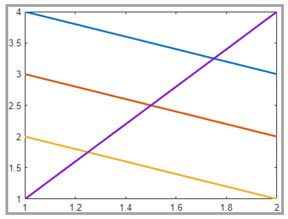
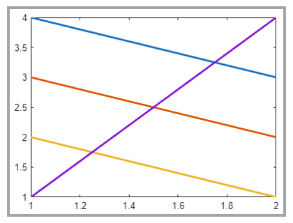
For example, create a line plot and export it as a 400-by-300-pixel JPG file using the default padding. The gray border around the image outlines the captured region. The border is not part of the saved image.

f = figure;
f.Position(3:4) = [400 300];
plot([4 3 2 1; 3 2 1 4],LineWidth=2)
exportgraphics(f,"plot-tight-padding.jpg", ...
       Units="pixels",Width=400,Height=300)

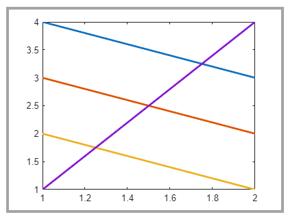
To use the same padding as displayed in the figure, specify the Padding name-value argument as "figure". The padding is included in the dimensions you specify. Therefore, the exported plot is slightly smaller to accommodate the extra padding.

exportgraphics(f,"plot-figure-padding.jpg", ...
       Units="pixels",Width=400,Height=300, ...
       Padding="figure")

To specify a custom padding value, specify the Padding name-value argument as a number in the same units as the Width and Height values. In this case, add 10 pixels to each side of the plot.

exportgraphics(f,"plot-10px-padding.jpg", ...
       Units="pixels",Width=400,Height=300, ...
       Padding=10)

Specify Background Color

By default, the exportgraphics function saves content with a background color that corresponds to the theme of the figure. You can specify a different background by setting the BackgroundColor name-value argument to one of these values:

• "current" — Select a color according to the color of the axes parent container (such as a figure or a panel). If the theme of the figure is light, then the background color is white. If the theme is dark, then the background color is dark gray (almost black). If the parent container has a custom color that you set, then the background color matches the custom color.

• "none" — Set the background color to transparent, white, or dark gray (almost black), depending on the value of ContentType:

  • When ContentType="vector", the background color is transparent.

  • When ContentType="image", the background color is white for light-themed figures, and dark gray (almost black) for dark-themed figures.

• A custom color, specified as an RGB triplet such as [1 0 0], a hexadecimal color code such as "#FF0000", or a named color such as "red".

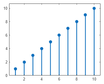
For example, create a stem plot and save the figure as a PDF file with a transparent background.

f = figure;
f.Position(3:4) = [400 300];
stem(1:10,"filled",LineWidth=2)
ylim padded
exportgraphics(f,"stem-transparent.pdf",ContentType="vector",...
               BackgroundColor="none")

Preserve Axes Limits and Tick Values

Occasionally, the exportgraphics function captures your content with different axes limits or tick values depending on the font size and the aspect ratio of the output. To keep the axes limits and tick values from changing, set the tick value mode and limit mode properties of the axes to "manual". For instance, when plotting into Cartesian axes, set the XTickMode, YTickMode, ZTickMode, XLimMode, YLimMode, and ZLimMode properties to "manual".

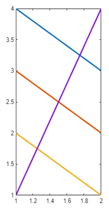
For example, this code creates a plot and sets the mode properties to "manual". Then it exports the plot with a significantly different aspect ratio. The axes limits and tick values are preserved in the output file.

f = figure;
f.Position(3:4) = [400 300];
plot([4 3 2 1; 3 2 1 4],LineWidth=2)

% Set the mode properties of the axes
ax = gca; 
ax.XTickMode = "manual";
ax.YTickMode = "manual";
ax.ZTickMode = "manual";
ax.XLimMode = "manual";
ax.YLimMode = "manual";
ax.ZLimMode = "manual";

exportgraphics(f,"eplot-preserveticks.png", ...
       Units="pixels",Width=200,Height=400)

For polar plots, set the RTickMode, ThetaTickMode, RLimMode, and ThetaLimMode properties of the polar axes to "manual".