Explore Boundary Model Types

Alternative Boundary Model Types

A boundary model describing the limits of the operating envelope can be useful when you are creating and evaluating designs, optimization results, and models.

Tip

You fit a boundary model by default when you use the Fit models common task button. Browse this page only if you want to explore alternative boundary model types.

• For one-stage models, the default boundary model is a Convex Hull fit to the inputs.

• For two-stage models, the default boundary model is a Convex Hull fit to the global inputs and a two-stage boundary model for the local input.

• For point-by-point models, the default is a separate boundary model of type Convex Hull to each operating point.

To edit existing boundary models or add new ones, from the test plan level, select TestPlan > Boundary Models, or the toolbar button Edit Boundary Models. The Boundary Editor appears.

In this editor, you can construct boundary models from your data. Boundary models are nonparametric surfaces you can use as a visual aid to understanding complex operating envelopes. You can use boundaries to guide modeling and constrain optimizations.

These boundary models are integrated with the rest of the toolbox. You can view them in the model plots and in CAGE in optimizations, tradeoff, model views, and the Surface Viewer. You can import boundary models into the Design Editor to use as constraints. You can also use them to clip models to view only the area of interest, to constrain models and designs to realistic engine operating envelopes, or to designate the most valid areas for optimization, tradeoff, and calibration.

• The toolbox saves boundary models implicitly as part of your test plan. You do not need to save them separately before closing the Boundary Editor.

• From the Boundary Editor, you can export boundary models to Simulink^®.

• From the Model Browser you can export boundary models with all your other models, from the test plan level. Use the File menu to export to CAGE, the Workspace or Simulink.

  For local boundary models only, export from the test plan by selecting TestPlan > Export Point-by-Point Models.

• You can use the function ceval to evaluate a boundary model exported to the Workspace. For example, if your exported model is M, then ceval(M, X) evaluates the boundary model attached to M at the points given by the matrix X (values less than zero are inside the boundary). See Evaluate Boundary Models in the Workspace for more details.

• You can import boundary models to use as constraints in the Design Editor.

Creating a New Boundary Model

You fit a boundary model by default when you use the Fit models common task button. To create a boundary model, leave the Fit boundary model check box selected in the Fit Models dialog box.

To edit existing boundary models or add new ones, from the Model Browser test plan level, select TestPlan > Boundary Models, or the toolbar button Edit Boundary Models. The Boundary Editor appears.

To create a boundary model:

1. In the Boundary Editor, get started by clicking New Boundary Model in the toolbar, or select File > New Boundary.

   You cannot access these options for leaf nodes. You can only add new boundary models at the root node and at the second-level nodes (local, global, or response).

2. For two-stage models, the Choose Level dialog box appears. Select a radio button to specify whether you want to model the boundary of the Local, Global, or Response values, and click OK.

   Note

   You can skip this step if you first select the Local, Global, or Response nodes in the Boundary Tree and then create a model. You get a new model appropriate for your current tree selection.

3. The controls available depend on the type of boundary model. See Setting Up Local, Global and Response Boundary Models.

After you create a boundary model, see Plotting Boundary Models.

Setting Up Local, Global and Response Boundary Models

• What Are Local, Global and Response Boundary Models?

• Setting Up Global and Response Boundary Models

• Setting Up Local Boundary Models

• Adding, Duplicating, and Deleting Boundary Models

What Are Local, Global and Response Boundary Models?

Response boundary models are built to cover the combination of the local and global variable spaces.

Global boundary models are built in the global variable space.

If you only select the global variables as active inputs to model, the differences between a global boundary model and a response boundary model are:

• For the response boundary model, the data includes all records.

• For the global boundary model, the data is one point per test (the average value of the global variables for that test).

Local boundary models fit the boundary of the local inputs. Local boundary models can be either two-stage or point-by-point global evaluation type.

• Two-stage boundary models fit the local boundary model parameters as a function of the global inputs. The toolbox uses an interpolating RBF for the function of the global inputs. For example, min_spark = f_1(speed, load) and max_spark = f_2(speed, load). This is useful for modeling borderline spark, for example.

  Two-stage boundaries are valid at any operating point.

• Point-by-point boundary models are separate boundary models fitted to the data collected at each operating point. Point-by-point boundary models are only valid at the observed operating points. The toolbox uses the global input values are used to select which local boundary model to use.

Setting Up Global and Response Boundary Models

When you set up a Global or Response boundary model, the Boundary Model Setup dialog box opens, displaying the controls shown in the following figure.

1. Select a type of boundary model: Range, Star-shaped, Ellipsoid, or Convex Hull.

   • The Range model finds the furthest extent of points for each variable and draws a hyper-rectangle to enclose all points.

     Range is the only type that you can use with only one input.

   • The Ellipsoid model forms an ellipse to enclose all points.

   • The Convex Hull model forms the minimal convex set containing the data points.

   • The Star-shaped model is a more complex model with various settings that determine how your boundary model is calculated. This calculation occurs in three stages: determining the center of the data; deciding which points are on the boundary, and interpolating between those points. The star-shaped model is the only model type that can fit non-convex regions.

2. Select a set of input factors to model using the Active Inputs check boxes. The required and selected number of inputs is displayed underneath. You might find it useful to build boundary models using subsets of input factors. You can then combine them for the most accurate boundary. This approach can be more effective than including all inputs.

3. The Fit Options tab is only enabled if your selected boundary type has any options you can set.

   • Range models do not have any further settings you can alter.

   • Star-shaped, convex hull, and ellipsoid models have several parameters that you can alter, see Editing Boundary Model Fit Options. Try the defaults before experimenting with these.

4. Click OK, and the toolbox calculates the boundary model.

Setting Up Local Boundary Models

For Local boundary models you can set up a two-stage boundary or a point-by-point boundary. When you set up a local boundary model, the Local Boundary Model Setup dialog box opens.

Two-Stage Boundaries.  To set up a two-stage boundary model:

1. Leave the default setting Two-stage in the Global evaluation list. You see the following controls.

   

2. You can select Range or Ellipsoid for the Local Boundary (to fit to the local inputs).

   You can select Ellipsoid only for more than one local variable. You can select Fit Options only for Ellipsoid models. Click Fit Options to see the parameters that you can alter. Try the defaults before experimenting with these. See Editing Boundary Model Fit Options.

3. The Global model must be an interpolating RBF that interpolates across the global inputs between these local boundaries. You can click Set Up to change the parameters for the interpolating RBF.

4. Click OK, and the toolbox calculates the boundary model.

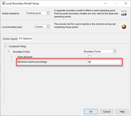
Point-by-Point Boundaries.  To set up a point-by-point boundary model:

1. Select Point-by-point in the Global evaluation list. You see the controls shown in the following figure.

   

2. Select the boundary settings. The available settings for point-by-point boundary models are the same as for global or response boundary models:

   1. Select a Local boundary type: Range, Star-shaped, Ellipsoid, or Convex Hull.

   2. Select a set of input factors to model using the Active Inputs check boxes.

   3. Optionally, view or edit settings on the Fit Options tab, if enabled for your boundary type.

   See Setting Up Global and Response Boundary Models for more details.

3. Click OK, and the toolbox calculates the boundary model.

Adding, Duplicating, and Deleting Boundary Models

• New boundary model (also in the File menu)— Opens a setup dialog box, and, when you click OK, adds a child node (containing a fitted boundary model) to the current node. This button is not enabled at leaf nodes. Similarly to the model tree in the Model Browser, the new child nodes are different depending on the location of your current selection in the tree.

  • For one-stage test plans, new child nodes of the root (top) node are boundary models (leaf nodes).

  • For two-stage test plans, new child nodes differ depending on the parent node. From the top or root node, you can choose a new child node of either local, global, or response type. From local, global, or response nodes, new child nodes are boundary models of the same type as their parent nod — local, global, or response. You can add as many boundary models of each type as you want.

• These toolbar buttons are only available for leaf nodes: (also in the Edit menu):

  • Duplicate boundary model — Duplicates the current node.

  • Delete boundary model — Deletes the current node.

Combining Best Boundary Models

You can select a single boundary model node as best or you can combine models by including them in your best selections. You might find it useful to build boundary models using subsets of inputs and different boundary types. You can then combine these models to achieve the most accurate boundary. This approach can be more effective than including all inputs.

Note

Only models selected as best are exported. Select one or more models as best, or you cannot export boundary models.

Look at the tree icons to see which boundary models are included as best. Included tree nodes have a check mark on their icon. In the following example, Response is included in best, and the child node Star-shaped is not included.

For two-stage or point-by-point test plans, the Local, Global, and Response nodes are included in best by default (even though they are empty to begin with). You can include or exclude any tree node except the root node.

Each parent node displays the combination of child nodes that you have selected as best (if any; otherwise the parent node is empty.) Use the toolbar and Edit menu items Add to Best and Remove From Best to include only the nodes you require at the root node.

For example, if you pick two leaf nodes and select Add to Best for each, the parent node shows a combination of the two boundary models. You might want your final model to combine boundaries of different types, e.g., a star-shaped and a range boundary. You can view the results at the parent node: the combined model is clipped to fit within the ranges defined by both boundaries. You can combine as many leaf nodes as you like.

Note

You can always see which boundaries have been combined at the currently selected node by viewing the Properties pane.

Use the following toolbar buttons or the Edit menu to combine and remove boundary models. These toolbar buttons are not available for the root node (only leaf and second-level nodes).

• Add to best — Include selected node in best. Only enabled where the selected node is excluded from best.

• Remove from best — Exclude selected node from best. Only enabled where the selected node is included in best.

You can combine the best models for one-stage or two-stage (local, global, and response) leaf nodes.

The Local node displays the child node or nodes selected as best (or is empty if none are selected as best). The Global and Response nodes also display their child node or combination of nodes selected as best. You can only combine local leaf nodes with other local leaf nodes, and global leaf nodes with other global leaf nodes, etc., because you can only have one best model at the Local node, one best model at the Global node, and one best model at the Response node. However you can choose to combine any of the Local, Global, or Response nodes as best for the root node. You can see which child model (or combination) is best from a parent node (e.g., Global) or the root node by looking under Best Boundary Model in the bottom left Properties pane.

See the following figure for an example.

In this example, the root node (DIVCP) is selected—the icon is outlined. Look at the Properties pane to see which leaf node (or nodes) you have included in the set of best boundary models for the selected node—in this case, it is Star-shaped (all inputs) and the Star-shaped(N,L) global nodes. The icons in the rest of the tree show the path of combined nodes.

Looking one level down in the tree, Local, Global, and Response are all included in best, but Local and Response are empty because they do not contain any child nodes selected as best. The Local and Response nodes are included in the best selection for the root node, but they have no effect because they are currently empty. Selections at different levels of the tree (branch and leaf) are independent.

Only the Global node contains any child nodes included in best, and therefore only that combination of global child nodes selected as best is displayed at the parent node (the root).

The Global node has the Star-shaped (all inputs) and the Star-shaped(N,L) child nodes selected as best. Therefore the Global node contains the combination of the Star-shaped (all inputs) and the Star-shaped(N,L) boundary models. The Global node is included in the best for the root node, so the root node also contains the Star-shaped (all inputs) and the Star-shaped(N,L) boundary models.

Editing Boundary Model Fit Options

To edit settings for existing boundary models, you can reach the Boundary Model Setup dialog boxes by selecting Edit > Set Up Boundary or the equivalent toolbar button, . This action opens the Boundary Model Setup dialog box where you can edit settings for the selected model. The new model is fitted when you click OK. You can edit the boundary type and active inputs, and settings where available.

You can view the type and details of the selected boundary model in the Properties pane. This pane displays information about the boundary model such as: number of data points; number of boundary, interior, and exterior points; the type of boundary model and summary of settings (e.g. center point of star). For root and branch nodes, you can see which model or combination of models you have selected as best.

See Combining Best Boundary Models for an example.

You can reach the Fit Options settings in the Boundary Model Setup dialog box, either when creating a boundary model, or when editing an existing boundary model, by selecting Edit > Set Up Boundary or the equivalent toolbar button.

The Fit Options tab (or button for local boundaries) is only enabled if your selected boundary type has any options you can set.

Range models have no additional settings you can alter.

Star-shaped, convex hull, and ellipsoid models have parameters that you can alter, as the following topics describe. Try the defaults before experimenting with these.

Ellipsoid Settings

The ellipsoid boundary has several optimization settings you can alter if you are having problems getting a good fit. Change the display setting to iter or final to see output messages at the command-line during the fit, and try different tolerances or numbers of iterations. For details on these settings see optimset in the MATLAB^® Reference.

Convex Hull Setting

The default convex hull boundary model keeps only the most useful facets and can discard around 30% of the facets that contribute only a small amount to the boundary. Discarding these facets is more efficient and includes all the data points within the boundary, with the total volume increasing by around 1%.

If you want the minimal volume at the expense of a much larger number of facets and a larger project file size, select the Keep All Facets check box. The total number of facets can be many thousands. In a typical example, using 8 factors and 70 points results in a convex hull with around 35,000 facets.

The convex hull is simplified to a range constraint when the volume is 99% of the box formed from the data range. You can change the Maximum volume percentage in the boundary editor. This reduces the number of linear constraints in CAGE optimizations when the data covers a rectangular region. A convex hull constraint is saved as a set of linear constraints, and prior to running optimizations in CAGE, the linear constraints are converted to bounds where possible.

Star-Shaped Settings

The Star-shaped boundary is a more complex model with various settings that determine how your boundary model is calculated. This determination occurs in three stages: determining the center of the data; deciding which points are on the boundary; and interpolating between those points.

• Special Points > Center — This setting is not the same as the Center Selection settings for RBFs, instead, the toolbox uses this setting as the method for determining the center of the boundary model sphere. Think of the boundary model as a deformed sphere. You can choose Mean, Median, Mid Range, MinEllipse or User Defined. If you select User Defined, you can enter a value for each input.

• Boundary Points — These settings determine how to decide which points are on the boundary.

  Interior — Choose this option to specify that not all points should be on the boundary.

  Boundary Only — Places all points on the boundary. This setting can save you time, if this is suitable for your data.

  • Dilation Radius — If you choose Interior points, then Dilation Radius is used to determine which points are on the boundary. The model-fitting calculation expands each point to a sphere until the intersection of all those spheres forms a boundary shape.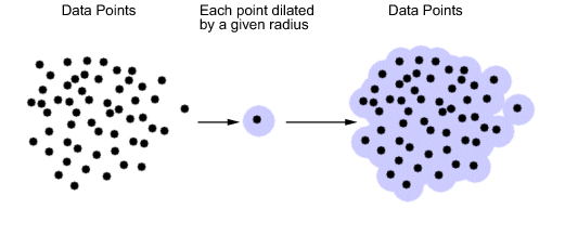

    

    Dilation Radius settings:

    • Auto — This setting selects the dilation radius (how much to expand each point) by checking all the minimum distances between points, and then choosing the largest of those.

    • Manual — You can manually set the dilation radius in the edit box. The default is 1. This value might seem large as model range is from -1 through 1, but all points are expanded equally so you will still detect the points on the edge. However, large spheres will intersect and obscure points that should be detected as boundary points.

  • Ray Casting — The toolbox draws rays from the center of the boundary model to determine which points are on the edge. The last point intersected on each ray is a boundary point. The ray actually intersects a sphere, given that the dilation radius expands the search point.

    

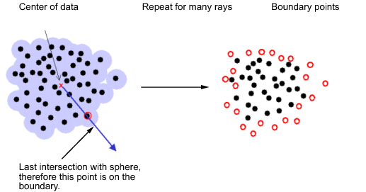
    Ray casting settings:

    • From Data — This option uses the same number of rays as there are data points and sends one ray in the direction of each point. If you have dense data or a large number of points, it might be better to use the Manual setting to choose a smaller number of rays.

    • Manual — You can set a value in the Number of Rays edit box. This number of rays is used in random directions. A good guideline is to use about twice the number of data points, although if you have a large number (many hundreds), the model fit becomes slow, and you might run out of memory. In most situations, more than 1000 is too many.

• Constraint Fit.

  • Transform — None, Log, or McCallum. The default is None. Depending on the shape of your boundary, you might need to use a transform to prevent self intersections near the center of the model.

  • RBF Kernel — Radial Basis Function (RBF) settings. You can choose RBF kernels, width, and continuity as when setting up models. See Global Model Class: Radial Basis Function for more information. After the boundary points have been determined, each of those points is used as an RBF center and the toolbox obtains the boundary surface by interpolating radial basis functions between all those centers. The width and continuity settings depend on which kernel you choose.

  • RBF Algorithm

    These options control the interpolating RBF model settings. You can leave the defaults unless you have a large data set (several thousand points). With large data sets, you can improve the speed and robustness of fitting if you try a different Algorithm setting, such as GMRES, first and then vary the tolerance and number of iterations.

Saving and Exporting Boundary Models

• File > Close — Closes the Boundary Editor and saves your boundary models with the test plan.

• File > Export to Simulink — Exports the currently selected node as a block in a Simulink model. If the currently selected node is a leaf node, the toolbox exports a single boundary model. If the selected node is a parent node (root, local, global, or response), the toolbox might export one boundary or a combination of several depending on which nodes you have assigned best and added to best.