Configure and Simulate LLC Resonant Converter Controller

R2026b

In this step of the LLC Resonant Converter Controller Design Workflow example, you can configure the plant model and controller gains for simulation. To get started, open the project and click the Configure and Simulate shortcut on the project toolstrip. The shortcut opens the live script so you can step through it..

In this stage you build the Simscape™ Electrical™ plant subsystem, configure the voltage controller subsystem reference with default or custom proportional-integral (PI) or 3-pole 3-zero (3p3z) gains, and validate the closed-loop response in simulation. The gains produced here are written to ctrlData.mat and are the starting point that every downstream stage of the project (frequency response estimation (FRE) tuning, stability analysis, hardware-in-the-loop (HIL) testing, hardware FRE, and algorithm export) consumes.

Configure Resonant Converter Plant

To make every downstream stage match your converter, first set the electrical parameters of the plant. The resonant converter electrical circuit is implemented as a plant model using Simscape Electrical and is parameterized through resonantconvertersimdata.m, which calls ResonantConv = PlantParameters('Converter100W');.

PlantParameters.m provides default LLC resonant converter parameters. To characterize a different converter, add a new case to the switch-case structure inside PlantParameters.m. Skip this section to continue with the default 100 W configuration.

edit PlantParameters; % Skip this section to proceed further with the default converter plant data.

After you add a new case, open resonantconvertersimdata.m and update the line below to select your custom converter name.

ResonantConv = PlantParameters('Converter100W');

The resonant converter plant model is implemented as a subsystem reference, so any parameter change here propagates directly into the closed-loop simulation model.

Note: The converter parameters defined here are reused by every later stage (closed-loop simulation, default-gain estimation, stability analysis, and frequency response analysis), so a single edit reconfigures the entire workflow.

Configure Resonant Converter Controller

To regulate the output voltage of the LLC resonant converter, the subsystem reference model at ~\ModelComponents\Controller\VoltageController.slx implements a voltage controller that uses direct frequency control of the resonant tank.

The controller supports two gain sets (default gains and custom gains), and the GainsSelector mask parameter picks between them at simulation time. Choosing the appropriate gain source lets you compare an analytically derived starting point against a hand-tuned or FRE-based design without editing the controller model.

Default Controller Gains

For the default gain calculation, the Resonant Converter Gains block uses the resonant converter parameters defined in the previous section and the controller sample time. When ResonantConverterSim.slx finishes a run, it writes these gains to ctrlData.mat, making them available to every downstream stage.

Custom Controller Gains

For custom gains, the Resonant Converter Gains block reads the values already stored in ctrlData.mat, so the controller runs against your overrides instead of the defaults.

To override the defaults, use the code below to write your own PI or higher-order compensator coefficients into ctrlData.mat. The kivoltTs field stores the integral gain pre-multiplied by the controller sample time, which lets the discrete-time integrator use a single multiply.

prjPath = matlab.project.rootProject().RootFolder;
matFile = fullfile(prjPath, 'Data', 'ctrlData.mat');
load(matFile); % Loads the structure ctrlData
ctrlData.Custom.kpvolt = 1100; % Kp for PI Control
ctrlData.Custom.kivoltTs = 70; % Ki*Ts
ctrlData.Custom.numecoef = [1 1 1]; % Coefficients for Higher order compensators
ctrlData.Custom.dencoef =  [1 1 1];%  Coefficients for Higher order compensators
ctrlData.Custom.ctrltype = 1; % 1 for PI 2 for Higher order compensators
ctrlData.Custom.timestamp =  datetime;
save(matFile, 'ctrlData');

Set ctrltype to 1 for a PI compensator or 2 for a 3-pole 3-zero (higher-order) compensator. The numecoef and dencoef fields are only used when ctrltype is 2. After the save completes, ctrlData.mat is the single source of truth for controller gains in every downstream stage.

Note: The gains stored in ctrlData.mat, whether default or custom, drive both the simulation and the stability analysis.

Simulate the Model

To validate that the plant model and controller work together before touching hardware, open and simulate ResonantConverterSim.slx. The simulation model consumes the parameters loaded in the previous stages and the two subsystem references: VoltageController and the converter plant. VoltageController contains the Resonant Converter Control Gains and Resonant Converter Controller blocks. The plant subsystem selects between half-bridge and full-bridge LLC topologies based on the PlantConfig field.

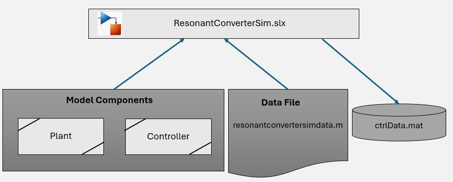
simmodel = ResonantConverterSim;
open_system(simmodel);

Run the open-loop simulation first to validate the plant model and the converter's electrical design. Confirm that the tank current, rectifier voltage, and DC output match your expectations. Then run the closed-loop simulation to validate the resonant controller design, the control gains, and the control-loop timing. Look for acceptable rise time, overshoot, and steady-state error at the reference voltage.

Note: To simulate a 3-pole 3-zero (3p3z) compensator instead of PI, use ResonantConverterSimHigherorder.slx. That model consumes the higher-order controller gains computed by CalcLlcType3CtrlGains and uses the same plant subsystem.