Estimate Online Frequency Response of LLC Resonant Converter

R2026b

In this step of the LLC Resonant Converter Controller Design Workflow example, you estimate the online frequency response of the LLC resonant converter plant to obtain a data-driven model for controller tuning. To get started, open the project and click the Online FRE shortcut on the project toolstrip. The shortcut opens this live script so you can step through it top to bottom.

This workflow extracts the plant frequency response of a resonant converter under open-loop control, enabling advanced control-gain estimation and stability analysis. The plant frequency response is defined as Vout/FreqIn and is obtained by modulating the open-loop control output with frequency perturbations. A well-conditioned frequency response estimation (FRE) result gives you a data-driven plant model that captures effects the analytical transfer function misses, including component nonlinearities, quantization, and topology-specific gain shaping around resonance.

The model references the plant subsystem from either HalfBridgeLLCConverter or FullBridgeLLCConverter. The model parameters are loaded from resonantconvertersimdata.m.

Configure FRE Injection Parameters

To characterize the plant across the control bandwidth without upsetting the operating point, define the sinestream perturbation. Choose a set of injection frequencies that spans the expected loop crossover, an amplitude that produces a measurable response while remaining in the linear regime, and enough settling and estimation periods for a clean estimate at each frequency. Configure the FRE parameters for your plant as follows:

• Amplitudes — Choose approximately 10% of the resonant frequency (for example, for a ~100 kHz resonant frequency, use ~10 kHz amplitude).

• FreqInjection — Limit the maximum injection frequency to 10% of the switching frequency (TsFre).

• NumSetPeriod — Increase if transients are observed and the system requires more time to settle.

FreqInjection        = [100 500 750 1000 1500 2000 3500 5000 10000 20000];%Hz Frequencies to be injected
Amplitudes  = 10000; % Amplitude of sine signals to be injected
NumSetPeriod = 4; % Number of settling periods for the frequency injection.
NumEstPeriod = 3; % Number of estimation periods for the frequency injection.
%Calculate simulation time to inject the frequencies
TestTime = 0;
for index = 1:length(FreqInjection)
    TestTime = TestTime + (NumSetPeriod+NumEstPeriod) / FreqInjection(index);    
end
TestTime = TestTime*1.01;

Simulate FRE Model

To capture how the plant gain shape changes across the operating envelope, sweep the open-loop switching frequency around resonance and estimate the plant at each point. The three chosen operating points (0.9*Fres, Fres, and 1.3*Fres) bracket the below-resonance, resonant, and above-resonance regions where the LLC gain characteristic differs most, so the controller can be tuned against the worst-case plant.

The step opens the OnlineFRESim model, applies the sinestream injection at each operating frequency, converts the estimated response into an frd object at the injected frequencies, and stores the result in FREDataStore. Saving the data store to llcplantfre.mat lets the stability and sensitivity analysis workflow reuse this data-driven plant without rerunning the simulation.

FreStartTime = 0.01;
SimTime1     = TestTime + FreStartTime;
fremodelname   = 'OnlineFRESim';
open_system(fremodelname);
resonantconvertersimdata; % Obtain the resonant converter data

FreFswOpenArray  = [ ResonantConv.Fres*0.9 ResonantConv.Fres ResonantConv.Fres*1.3] ;% Open loop switching frequency.
Fieldtags = arrayfun(@(k) sprintf('F%d', k), 1:numel(FreFswOpenArray), 'UniformOutput', false); % Field tags {'F1', 'F2', 'F3' ..}

FREDataStore =  struct();



for ite =1:length(FreFswOpenArray)
    FREFswOpen = FreFswOpenArray(ite);
    sim(fremodelname);
    FREDataStore.(Fieldtags{ite}).FRE = frd(FRD.Data, FreqInjection * 2 * pi); % Create frequency response data object
    FREDataStore.(Fieldtags{ite}).FswOpenloop = FreFswOpenArray(ite);
end

% Store the frequency response data for each frequency
rootFolder = currentProject().RootFolder;
save (rootFolder+'\Data\llcplantfre.mat',"FREDataStore");

After the sweep, FREDataStore contains one frd object per operating point. Any distortion, missing samples, or unexpected magnitude jumps in these estimates usually points to an amplitude that is too large, too few settling periods, or a frequency injected outside the linear range. Re-tune Amplitudes or NumSetPeriod before proceeding.

Plot the FRE

To confirm that the estimated plant behavior matches expectations for a resonant converter, overlay the Bode magnitude and phase of the three operating points. Setting FreqUnits to Hz and constraining XLim to [100 1e5] focuses the view on the control-relevant decade where the loop crossover sits.

fields = fieldnames(FREDataStore);
legendEntries = cell(1, numel(fields));
for k = 1:numel(fields)
    fsw = FREDataStore.(fields{k}).FswOpenloop;
    legendEntries{k} = sprintf('Fsw = %.1f kHz', fsw/1e3);
end

bodeOpts = bodeoptions;
bodeOpts.FreqUnits = 'Hz';
bodeOpts.Grid = 'on';
bodeOpts.XLim = {[100 1e5]}; 

figure;
bodeplot(FREDataStore.F1.FRE, FREDataStore.F2.FRE, FREDataStore.F3.FRE, bodeOpts);
legend(legendEntries, 'Location', 'best');
title('LLC Plant FRE Bode Plot');

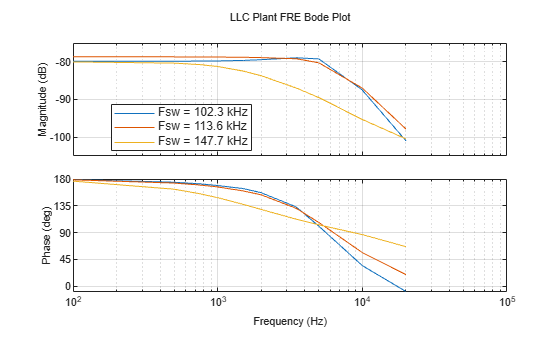
The traces should show smooth magnitude and phase curves that shift with operating frequency: gain is highest near resonance and drops as the switching frequency moves above Fres. Sudden discontinuities or noisy samples at low frequencies typically indicate that NumSetPeriod and NumEstPeriod need to be increased so the response has time to reach steady state.

Plot FRE and Analytical TF

Validate the data-driven plant against the analytical transfer function at each operating point.

%% Overlay TF on FRE Bode
freSys = cell(1, numel(Fieldtags)); % Preallocate array with size equal to field tags
tfSys  = cell(1, numel(Fieldtags));
legendAll = cell(1, 2*numel(Fieldtags));

for k = 1:numel(Fieldtags)
    freSys{k} = FREDataStore.(Fieldtags{k}).FRE; % Store the FRE models with field tags {'F1', 'F2', 'F3' ..}
    legendAll{k} = sprintf('FRE  %.1f kHz', FreFswOpenArray(k)/1e3);

    Foperate = FreFswOpenArray(k) / ResonantConv.Fres;
    [Gp, ~] = buildPlantFromTopology(ResonantConv, Foperate); % Get plant transfer function at the operating point
    tfSys{k} = Gp;
    legendAll{numel(Fieldtags)+k} = sprintf('TF   %.1f kHz', FreFswOpenArray(k)/1e3);
end

figure;
bodeplot(freSys{:}, tfSys{:}, bodeOpts);
legend(legendAll, 'Location', 'best');
title('LLC Plant: FRE vs Analytical TF');

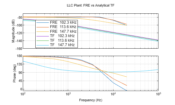
The overlay shows the two models track closely at low frequency, through the DC gain, the output-filter pole, and the equivalent series resistance (ESR) zero, and then diverge at high frequencies, near resonance and the switching and sampling dynamics. The small-signal transfer function captures the low-frequency behavior that sets the loop crossover. Therefore, it is a good starting point for controller design. Deriving the PI gains against the analytical transfer function gives the margins in the desirable range without an FRE estimate. At higher frequencies, where the two models diverge, the FRE covers the effects of the transport delay, sampling, and near-resonance dynamics that the averaged model smooths away. Initial compensator design using the analytical TF gives a good starting point for converter control. Rely on the FRE-based plant, especially for controller goals of higher bandwidth or crossover frequency.