Use MPC with Extended State Observer to Reject Unmeasured Output Disturbances

This example shows how to combine MPC with an extended state observer to reject unmeasured disturbance at the plant output.

Understand Built-In Disturbance Rejection of MPC Controller

Given initial states and a sequence of control actions, a dynamic model can be used to describe the behavior of the plant across the prediction horizon. Based on this dynamic model, an MPC controller can find an optimal control sequence that minimizes reference tracking errors and reduces control efforts by solving a constrained optimization problem at each control interval.

For this example, define a continuous-time, single-input, single-output linear plant with two states.

G = ss([-2 1;-9.7726 -1.3863],[0;1],[0.5 0],0);

Design a linear MPC controller for reference tracking with a sample time of 0.1 second.

Ts = 0.1;
c = mpc(G, Ts);

-->"PredictionHorizon" is empty. Assuming default 10.
-->"ControlHorizon" is empty. Assuming default 2.
-->"Weights.ManipulatedVariables" is empty. Assuming default 0.00000.
-->"Weights.ManipulatedVariablesRate" is empty. Assuming default 0.10000.
-->"Weights.OutputVariables" is empty. Assuming default 1.00000.

For this example, also assume that the plant is derived by linearizing a nonlinear plant around a specific operating point. Specify the state, input, and output values of the operating point in MPC as its nominal values.

x0 = [1.6931; 4.3863];
u0 = 7.7738;
y0 = 0.5;
c.Model.Nominal.Y = y0;
c.Model.Nominal.U = u0;
c.Model.Nominal.X = x0;

By default, the MPC controller provides a built-in mechanism to help reject unmeasured output disturbance. Specifically, this mechanism consists of a default output disturbance model that has integrators with a dimensionless unity gain added to some or all of its outputs. To study how MPC reacts to modeling errors and unmeasured disturbances, disable this mechanism by setting the output disturbance model to an unit gain.

% Remove default output disturbance model.
setoutdist(c,"model",tf(0));            

As a consequence, the plant used for simulation is identical to the prediction model. Simulate a 5-second closed-loop response that tracks a step change of 0.1 in the reference output.

% Set number of steps for simulation time of 5 seconds.
SimulationSteps = 51;      

% Define Reference signal.
ref = y0+0.1*ones(SimulationSteps,1);

% Run closed-loop simulation.
[y, t] = sim(c,SimulationSteps,ref);

-->Converting model to discrete time.
-->"Model.Noise" is empty. Assuming white noise on each measured output.

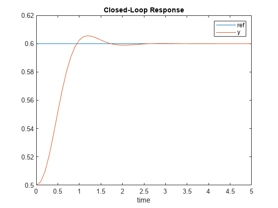
Plot the closed loop response.

plot(t,ref,t,y);
xlabel('time');
title('Closed-Loop Response');
legend('ref','y');

Since the MPC prediction model and the plant used for simulation are identical, the controller is able to bring plant output to its new reference value, achieving zero steady state error.

In the real world, however, modeling errors are likely. To examine the impact of modeling error on the closed-loop performance, set the plant used for simulation to G*2 (a different DC gain).

% Get default simulation options object.
opt = mpcsimopt;

% Specify plant used for simulation.
opt.Model = G*2;

% Run closed-loop simulation.
[y, t] = sim(c,SimulationSteps,ref,opt);

-->Converting model to discrete time.

Plot the closed loop response.

plot(t,ref,t,y);
xlabel('time');
title('Closed-Loop Response');
legend('ref','y');

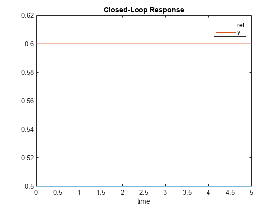
Because of the modeling error, the plant output now has a nonzero steady-state error.

Consider now another scenario where instead of a modeling error, you have a constant unmeasured output disturbance occurring at the plant output. Simulate this scenario to see how the controller handles disturbances. The reference signal remains unchanged.

% Create simulation options object.
opt = mpcsimopt;

% Specify output disturbance of 0.1.
opt.OutputNoise = 0.1;       

% Display measured plant output (disturbance included).
opt.ShowOutputNoise = true;

% Define reference signal.
ref = y0*ones(SimulationSteps,1);  

% Perform closed-loop simulation.
[y, t, u, x_plant] = sim(c,SimulationSteps,ref,opt);
plot(t,ref,t,y);
xlabel('time');
title('Closed-Loop Response');
legend('ref','y');

The controller is not able to keep the output at its reference value, that is, it fails to reject the output disturbance. This is not surprising because MPC is not aware of the existence of the disturbance. Since the built-in Kalman filter accurately estimates the plant states, MPC maintains the output of the plant model at the reference of 0.5 even though the real plant output is 0.6.

Display the output of the MPC internal plant model at the end of simulation.

G.C*(x_plant(end,:)'-x0)+y0

ans = 
0.5000

In summary, you have two choices to achieve disturbance rejection with MPC:

• If MPC knows about what kind of disturbance is expected and the disturbance is estimated at run time, MPC should be able to reject it;

• If MPC does not have any knowledge of the disturbance, you must implement an additional disturbance rejection mechanism to assist MPC.

The remaining part of this example shows how to use the Extended State Observer block from Simulink® Control Design™ to work with MPC for disturbance rejection.

MPC with Extended State Observer

For MPC to perform disturbance rejection, it must know about the disturbance and how it impacts the plant. One general way to do this is to use a disturbance model to describe the nature of the disturbance, augment the plant model with the disturbance model, and then use state estimation techniques to provide states of the overall model at run time. For example, if you expect a step-like disturbance occurring at the plant output, the disturbance model is simply an integrator whose input is white noise with zero mean and variance one. The output of the integrator reflects the estimated disturbance amplitude at run time. Since MPC ensures that the sum of the plant model output and the disturbance model output track the reference signal, it achieves disturbance rejection.

This is exactly what the default MPC design does for you. Revert MPC to use the default output disturbance model, which is a discrete-time integrator.

% Revert to the default output disturbance model
setoutdist(c,'integrators');

% Display the disturbance model.
tf(getoutdist(c))

-->Converting model to discrete time.
-->Assuming output disturbance added to measured output #1 is integrated white noise.
-->"Model.Noise" is empty. Assuming white noise on each measured output.

ans =
 
  From input to output "MO1":
   0.1
  -----
  z - 1
 
Sample time: 0.1 seconds
Discrete-time transfer function.

The integrator as disturbance model compensates for step-like disturbances. If you expect a different type of disturbance, you can use a custom disturbance model to describe your expected disturbance. For example, if the disturbance is a ramp-like signal, set the output disturbance model to a double integrator.

After you augment the plant model with the disturbance model, a built-in Kalman filter is automatically designed for the overall system such that the plant states and the disturbance model state can be estimated at run time based on the measured plant output. For more information on how default Kalman gains are calculated, see Implement Custom State Estimator Equivalent to Built-In Kalman Filter.

If the default Kalman filter does not lead to satisfactory observer performance, you can customize it. One approach is to use the setEstimator command to directly edit Kalman gains. The other approach is to use a custom state observer outside MPC and feed estimated states (instead of measured plant output) to MPC at run time. The second approach decouples MPC from state estimation and gives you maximum flexibility to design a custom state observer.

The remaining part of this example shows how to use an extended state observer (ESO) as an alternative to the built-in Kalman filter.

Consider the following plant model:

.

An extended state observer is able to estimate the disturbance $\mathit{d}$ and system state $\mathit{x}$ based on the measured system input $\mathit{u}$ and output $\mathit{y}$ at run time.

For the ESO to work properly, disturbance $\mathit{d}$ must have a direct impact on the system state. However, since the additive disturbance occurring at the plant output does not impact plant state, you cannot use the plant model directly in the ESO. Fortunately, the augmented model used by the previous Kalman filter design can serve as the system in ESO, where both the plant state and the disturbance model state are parts of the system state in the ESO and the white noise becomes the input $\mathit{d}$ in the ESO. When you use this ESO together with MPC, the estimated state from the ESO can be directly fed to MPC while the estimated $\mathit{d}$ is discarded.

To design a discrete-time ESO for the MPC used in this example, follow these steps.

First, configure the overall system model, Geso.

% Obtain discrete-time plant model.
Gp = c2d(G,Ts);

% Obtain discrete-time output disturbance model (an integrator).
Gd = getoutdist(c);

% Combine to form the overall system and produce A, Bu and Cm.
A = blkdiag(Gp.A, Gd.A);
Bu = [Gp.B; 0];
Cm = [Gp.C Gd.C];
Geso = ss(A,Bu,Cm,0,Ts);

Second, since the "white noise" input $\mathit{d}$ only impacts the last state in $\mathit{Geso}$, set the disturbance input matrix $\mathit{Bd}$ to [0;0;1].

Bd = [0;0;1];

Third, design the observer gain, $\mathit{L}$, using pole placement.

% Define number of states (2 from plant and 1 from disturbance model).
nx = 3;
% Define number of disturbances (1 from disturbance model input).
nd = 1;
% Define number of outputs.
ny = 1;
% Specify observer bandwidth (rad/s).
wo = 2;
% Specify space between poles (rad/s).
space = 1;

% Calculate discrete-time pole locations.
poles = exp(-wo*(1:space:1+space*(nx+nd-1))*Ts);

% Calculate observer gain using pole placement.
C_hat = [Geso.C,zeros(ny,nd)];
A_hat = [Geso.A,Bd;zeros(nd,nx),eye(nd,nd)];
L = place(A_hat',A_hat'*C_hat',poles)';

In the Simulink model, you can compare the performance between two MPC controllers. They both use the same overall prediction model (that is, a plant model augmented with an output disturbance model) with one using the built-in Kalman filter for state estimation and the other using the designed ESO.

mdl = 'mpc_ExtendedStateObserver';
open_system(mdl);

The ESO block, available in Simulink Control Design, receives $\mathit{Bd}$ and $\mathit{L}$ matrices from two constant blocks (as external sources) and the system model Geso is defined in the block dialog.

Two MPC controllers, c and cESO, are the same except the one working with ESO is configured to use custom estimation.

cESO = c;
setEstimator(cESO,'custom');

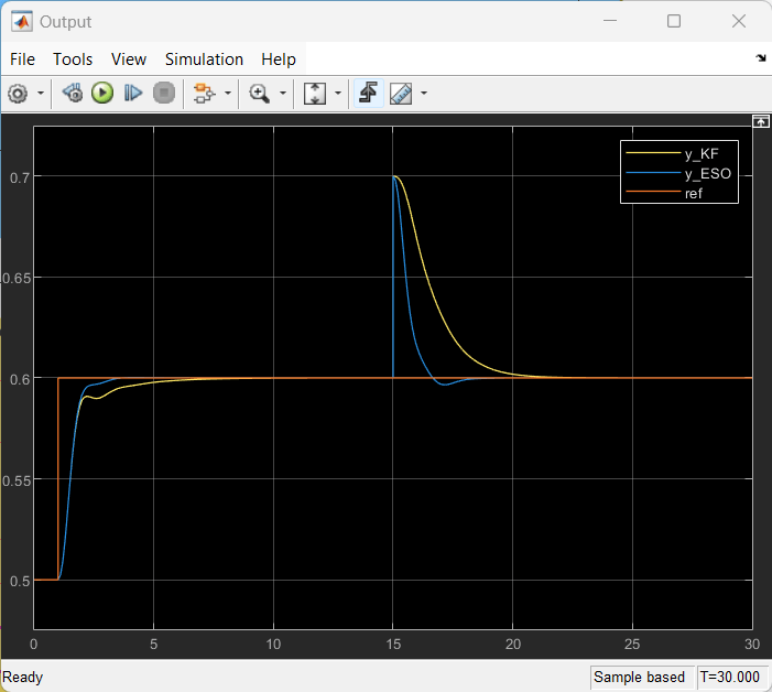
Simulate and compare the closed-loop performance for reference tracking (at 1 second) and output disturbance rejection (at 15 second).

sim(mdl);

-->Converting model to discrete time.
-->Assuming output disturbance added to measured output #1 is integrated white noise.
-->"Model.Noise" is empty. Assuming white noise on each measured output.

In this case, since ESO provides faster state estimation than the built-in Kalman filter, MPC with ESO is able to respond faster to reference tracking and disturbance rejection demands.