stuffABCD
Description
Examples
Define delta-sigma modulator parameters.
order = 5;      % Modulator order
OSR = 32;       % Oversampling ratio
N = 8192;       % Number of simulation points
f = 85;         % Input signal frequency bin
amp = 0.5;      % Input signal amplitude (should be less than 1)
fB = ceil(N/(2*OSR));
Create a sinusoidal input signal.
u = amp * sin(2*pi*f/N * (0:N-1)) % Create a sine wave inputu = 1×8192
0 0.0326 0.0650 0.0972 0.1289 0.1601 0.1906 0.2203 0.2491 0.2768 0.3034 0.3286 0.3525 0.3748 0.3956 0.4147 0.4320 0.4475 0.4611 0.4727 0.4823 0.4899 0.4953 0.4987 0.5000 0.4991 0.4961 0.4911 0.4839 0.4746 0.4634 0.4502 0.4350 0.4181 0.3993 0.3789 0.3568 0.3332 0.3082 0.2819 0.2544 0.2258 0.1963 0.1659 0.1348 0.1032 0.0711 0.0387 0.0061 -0.0264
Synthesize the noise transfer function (NTF).
H = synthesizeNTF(order, OSR, 1)
H =

         (z-1) (z^2 - 1.997z + 1) (z^2 - 1.992z + 1)
  ----------------------------------------------------------
  (z-0.7778) (z^2 - 1.613z + 0.6649) (z^2 - 1.796z + 0.8549)

Sample time: 1 seconds
Discrete-time zero/pole/gain model.
Model Properties
Realize the NTF into coefficients for a CRFB modulator structure.
[a, g, b, c] = realizeNTF(H, 'CRFB')a = 1×5
0.0007 0.0084 0.0550 0.2443 0.5579
g = 1×2

    0.0028    0.0079
b = 1×6

    0.0007    0.0084    0.0550    0.2443    0.5579    1.0000
c = 1×5

     1     1     1     1     1
Assemble the final ABCD matrix.
ABCD = stuffABCD(a, g, b, c, 'CRFB')ABCD = 6×7
1.0000 0 0 0 0 0.0007 -0.0007
1.0000 1.0000 -0.0028 0 0 0.0084 -0.0084
1.0000 1.0000 0.9972 0 0 0.0633 -0.0633
0 0 1.0000 1.0000 -0.0079 0.2443 -0.2443
0 0 1.0000 1.0000 0.9921 0.8023 -0.8023
0 0 0 0 1.0000 1.0000 0
Run the simulation.
[v,xn,xmax,y] = simulateDSM(u, ABCD)
v = 1×8192

     1    -1    -1     1     1    -1     1    -1     1     1    -1     1     1     1    -1     1     1    -1     1    -1     1     1     1     1     1    -1     1    -1     1     1     1     1     1    -1     1     1    -1     1    -1     1    -1     1     1     1    -1    -1     1     1    -1     1
xn = 5×8192

   -0.0007    0.0000    0.0007    0.0001   -0.0005    0.0003   -0.0002    0.0006    0.0001   -0.0004    0.0005    0.0000   -0.0004   -0.0008    0.0001   -0.0003   -0.0007    0.0003   -0.0000    0.0009    0.0006    0.0003   -0.0001   -0.0004   -0.0008    0.0002   -0.0001    0.0009    0.0006    0.0002   -0.0002   -0.0005   -0.0009    0.0001   -0.0004   -0.0008    0.0001   -0.0003    0.0006    0.0001    0.0009    0.0004   -0.0001   -0.0007    0.0001    0.0008    0.0002   -0.0005    0.0002   -0.0005
   -0.0084   -0.0002    0.0087    0.0017   -0.0055    0.0039   -0.0026    0.0075    0.0016   -0.0044    0.0062    0.0010   -0.0045   -0.0100    0.0010   -0.0038   -0.0087    0.0029   -0.0013    0.0111    0.0075    0.0036   -0.0004   -0.0047   -0.0092    0.0028   -0.0013    0.0112    0.0075    0.0035   -0.0008   -0.0056   -0.0108    0.0004   -0.0046   -0.0100    0.0008   -0.0047    0.0061    0.0006    0.0112    0.0054   -0.0010   -0.0081    0.0009    0.0102    0.0031   -0.0049    0.0032   -0.0053
   -0.0633   -0.0068    0.0604    0.0126   -0.0407    0.0269   -0.0202    0.0544    0.0147   -0.0294    0.0484    0.0125   -0.0276   -0.0720    0.0058   -0.0302   -0.0701    0.0124   -0.0185    0.0735    0.0525    0.0281   -0.0001   -0.0323   -0.0690    0.0161   -0.0128    0.0803    0.0595    0.0341    0.0038   -0.0320   -0.0738    0.0046   -0.0330   -0.0772   -0.0019   -0.0431    0.0349   -0.0040    0.0761    0.0390   -0.0061   -0.0600    0.0032    0.0741    0.0261   -0.0316    0.0269   -0.0348
   -0.2443   -0.0490    0.2066    0.0423   -0.1585    0.0888   -0.0833    0.1978    0.0647   -0.0984    0.1934    0.0734   -0.0745   -0.2534    0.0218   -0.1157   -0.2814    0.0102   -0.1075    0.2386    0.1820    0.1070    0.0104   -0.1113   -0.2619    0.0435   -0.0623    0.2931    0.2423    0.1688    0.0682   -0.0641   -0.2330    0.0452   -0.0982   -0.2807   -0.0191   -0.1825    0.0998   -0.0416    0.2637    0.1457   -0.0142   -0.2231    0.0006    0.2749    0.1164   -0.0948    0.1221   -0.1046
   -0.8023   -0.2752    0.5256    0.0641   -0.5804    0.1557   -0.3792    0.4995    0.1453   -0.3567    0.5640    0.2627   -0.1730   -0.7752    0.0252   -0.4171   -1.0153   -0.1975   -0.6057    0.4545    0.3477    0.1701   -0.1011   -0.4921   -1.0330   -0.1531   -0.4965    0.6285    0.5829    0.4586    0.2274   -0.1435   -0.6917    0.1447   -0.2887   -0.9159   -0.1781   -0.7326    0.0971   -0.3451    0.6185    0.3323   -0.1304   -0.8189   -0.1851    0.7052    0.3034   -0.3277    0.3557   -0.3216
xmax = 5×1

    0.0014
    0.0167
    0.1147
    0.3735
    1.1084
y = 1×8192

         0   -0.7697   -0.2102    0.6227    0.1930   -0.4203    0.3463   -0.1588    0.7486    0.4221   -0.0533    0.8926    0.6152    0.2018   -0.3796    0.4399    0.0149   -0.5679    0.2635   -0.1330    0.9368    0.8375    0.6654    0.3977    0.0079   -0.5338    0.3431   -0.0054    1.1124    1.0575    0.9220    0.6776    0.2916   -0.2736    0.5440    0.0902   -0.5591    0.1551   -0.4244    0.3790   -0.0907    0.8443    0.5286    0.0355   -0.6841   -0.0820    0.7763    0.3421   -0.3216    0.3293
Analyze the output.
figure;
spec = fft(v .* ds_hann(N)) / (N/4);
plot(dbv(spec));
axis([0 N/2 -120 0]);
title('Spectrum of Modulator Output');
xlabel('Frequency Bin');
ylabel('dBV');
grid on;
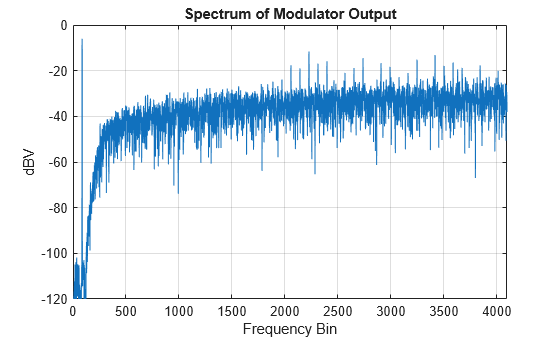
Calculate SNR.
snr = calculateSNR(spec(1:fB),f)
snr =
82.5313
Calculate the NTF and STF of the modulator.
[ntf,stf] = calculateTF(ABCD,1)
ntf =

         (z-1) (z^2 - 1.997z + 1) (z^2 - 1.992z + 1)
  ----------------------------------------------------------
  (z-0.7778) (z^2 - 1.613z + 0.6649) (z^2 - 1.796z + 0.8549)

Sample time: 1 seconds
Discrete-time zero/pole/gain model.
Model Properties

stf =

  1

Static gain.
Model Properties
Map the ABCD matrix back to coefficients of the CRFB topology.
[a,g,b,c] = mapABCD(ABCD,'CRFB')a = 1×5
0.0007 0.0084 0.0550 0.2443 0.5579
g = 1×2

    0.0028    0.0079
b = 1×6

    0.0007    0.0084    0.0550    0.2443    0.5579    1.0000
c = 1×5

     1     1     1     1     1
Dynamically scale the ABCD matrix so that the state maxima are less than specified limit 1.
nlev = 2;
xlim = 1;
ymax = nlev+5;
[ABCDs,umax]=scaleABCD(ABCD,nlev,f,xlim,ymax,N)
ABCDs = 6×7

    1.0000         0         0         0         0   -0.0007    0.0007
    1.0000    1.0000   -0.0028         0         0   -0.0084    0.0084
    1.0000    1.0000    0.9972         0         0   -0.0633    0.0633
         0         0    1.0000    1.0000   -0.0079   -0.2443    0.2443
         0         0    1.0000    1.0000    0.9921   -0.8023    0.8023
         0         0         0         0   -1.0000    1.0000         0
umax =
8192
Input Arguments
Output Arguments
Version History
Introduced in R2026a
See Also
calculateTF | synthesizeNTF | realizeNTF | mapABCD | scaleABCD | predictSNR | calculateSNR | simulateSNR | simulateDSM