Tutorial for Optimization Toolbox

This tutorial includes multiple examples that show how to use two nonlinear optimization solvers, fminunc and fmincon, and how to set options. The principles outlined in this tutorial apply to the other nonlinear solvers, such as fgoalattain, fminimax, lsqnonlin, lsqcurvefit, and fsolve.

The tutorial examples cover these tasks:

• Minimizing an objective function

• Minimizing the same function with additional parameters

• Minimizing the objective function with a constraint

• Obtaining a more efficient or accurate solution by providing gradients or a Hessian, or by changing options

Unconstrained Optimization Example

Consider the problem of finding a minimum of the function

$$x\exp (-(x^2+y^2))+(x^2+y^2)/20.$$

Plot the function to see where it is minimized.

f = @(x,y) x.*exp(-x.^2-y.^2)+(x.^2+y.^2)/20;
fsurf(f,[-2,2],'ShowContours','on')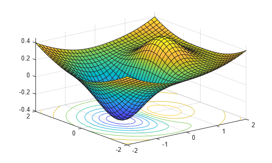

The plot shows that the minimum is near the point (–1/2,0).

Usually you define the objective function as a MATLAB® file. In this case, the function is simple enough to define as an anonymous function.

fun = @(x) f(x(1),x(2));

Set an initial point for finding the solution.

x0 = [-.5; 0];

Set optimization options to use the fminunc default 'quasi-newton' algorithm. This step ensures that the tutorial works the same in every MATLAB version.

options = optimoptions('fminunc','Algorithm','quasi-newton');

View the iterations as the solver performs its calculations.

options.Display = 'iter';

Call fminunc, an unconstrained nonlinear minimizer.

[x, fval, exitflag, output] = fminunc(fun,x0,options);

                                                        First-order 
 Iteration  Func-count       f(x)        Step-size       optimality
     0           3          -0.3769                         0.339
     1           6        -0.379694              1          0.286  
     2           9        -0.405023              1         0.0284  
     3          12        -0.405233              1        0.00386  
     4          15        -0.405237              1       3.17e-05  
     5          18        -0.405237              1       3.35e-08  

Local minimum found.

Optimization completed because the size of the gradient is less than
the value of the optimality tolerance.

<stopping criteria details>

Display the solution found by the solver.

uncx = x

uncx = 2×1

   -0.6691
    0.0000

View the function value at the solution.

uncf = fval

uncf = 
-0.4052

The examples use the number of function evaluations as a measure of efficiency. View the total number of function evaluations.

output.funcCount

ans = 
18

Unconstrained Optimization Example with Additional Parameters

Next, pass extra parameters as additional arguments to the objective function, first by using a MATLAB file, and then by using a nested function.

Consider the objective function from the previous example.

$$f(x,y)=x\exp (-(x^2+y^2))+(x^2+y^2)/20.$$

Parameterize the function with (a,b,c) as follows:

$$f(x,y,a,b,c)=(x-a)\exp (-((x-a{)}^2+(y-b{)}^2))+((x-a{)}^2+(y-b{)}^2)/c.$$

This function is a shifted and scaled version of the original objective function.

MATLAB File Function

Consider a MATLAB file objective function named bowlpeakfun defined as follows.

type bowlpeakfun

function y = bowlpeakfun(x, a, b, c)
%BOWLPEAKFUN Objective function for parameter passing in TUTDEMO.

%   Copyright 2008 The MathWorks, Inc.

y = (x(1)-a).*exp(-((x(1)-a).^2+(x(2)-b).^2))+((x(1)-a).^2+(x(2)-b).^2)/c;

Define the parameters.

a = 2;
b = 3;
c = 10;

Create an anonymous function handle to the MATLAB file.

f = @(x)bowlpeakfun(x,a,b,c)

f = function_handle with value:
    @(x)bowlpeakfun(x,a,b,c)

Call fminunc to find the minimum.

x0 = [-.5; 0];
options = optimoptions('fminunc','Algorithm','quasi-newton');
[x, fval] = fminunc(f,x0,options)

Local minimum found.

Optimization completed because the size of the gradient is less than
the value of the optimality tolerance.

<stopping criteria details>

x = 2×1

    1.3639
    3.0000

fval = 
-0.3840

Nested Function

Consider the nestedbowlpeak function, which implements the objective as a nested function.

type nestedbowlpeak

function [x,fval] =  nestedbowlpeak(a,b,c,x0,options)
%NESTEDBOWLPEAK Nested function for parameter passing in TUTDEMO.

%   Copyright 2008 The MathWorks, Inc.

[x,fval] = fminunc(@nestedfun,x0,options);  
    function y = nestedfun(x)
      y = (x(1)-a).*exp(-((x(1)-a).^2+(x(2)-b).^2))+((x(1)-a).^2+(x(2)-b).^2)/c;    
    end
end

The parameters (a,b,c) are visible to the nested objective function nestedfun. The outer function, nestedbowlpeak, calls fminunc and passes the objective function, nestedfun.

Define the parameters, initial guess, and options:

a = 2;
b = 3;
c = 10;
x0 = [-.5; 0];
options = optimoptions('fminunc','Algorithm','quasi-newton');

Run the optimization:

[x,fval] =  nestedbowlpeak(a,b,c,x0,options)

Local minimum found.

Optimization completed because the size of the gradient is less than
the value of the optimality tolerance.

<stopping criteria details>

x = 2×1

    1.3639
    3.0000

fval = 
-0.3840

Both approaches produce the same answers, so you can use the one you find most convenient.

Constrained Optimization Example: Inequalities

Consider the previous problem with a constraint:

$$\text{minimize}x\exp (-(x^2+y^2))+(x^2+y^2)/20,$$

$$\text{subject}\text{to}xy/2+(x+2{)}^2+(y-2{)}^2/2\le 2.$$

The constraint set is the interior of a tilted ellipse. View the contours of the objective function plotted together with the tilted ellipse.

f = @(x,y) x.*exp(-x.^2-y.^2)+(x.^2+y.^2)/20;
g = @(x,y) x.*y/2+(x+2).^2+(y-2).^2/2-2;
fimplicit(g)
axis([-6 0 -1 7])
hold on
fcontour(f)
plot(-.9727,.4685,'ro');
legend('constraint','f contours','minimum');
hold off

The plot shows that the lowest value of the objective function within the ellipse occurs near the lower-right part of the ellipse. Before calculating the plotted minimum, make a guess at the solution.

x0 = [-2 1];

Set optimization options to use the interior-point algorithm and display the results at each iteration.

options = optimoptions('fmincon','Algorithm','interior-point','Display','iter');

Solvers require that nonlinear constraint functions give two outputs, one for nonlinear inequalities and one for nonlinear equalities. To give both outputs, write the constraint using the deal function.

gfun = @(x) deal(g(x(1),x(2)),[]);

Call the nonlinear constrained solver. The problem has no linear equalities or inequalities or bounds, so pass [ ] for those arguments.

[x,fval,exitflag,output] = fmincon(fun,x0,[],[],[],[],[],[],gfun,options);

                                            First-order      Norm of
 Iter F-count            f(x)  Feasibility   optimality         step
    0       3    2.365241e-01    0.000e+00    1.972e-01
    1       6    1.748504e-01    0.000e+00    1.734e-01    2.260e-01
    2      10   -1.570560e-01    0.000e+00    2.608e-01    9.347e-01
    3      14   -6.629160e-02    0.000e+00    1.241e-01    3.103e-01
    4      17   -1.584082e-01    0.000e+00    7.934e-02    1.826e-01
    5      20   -2.349124e-01    0.000e+00    1.912e-02    1.571e-01
    6      23   -2.255299e-01    0.000e+00    1.955e-02    1.993e-02
    7      26   -2.444225e-01    0.000e+00    4.293e-03    3.821e-02
    8      29   -2.446931e-01    0.000e+00    8.100e-04    4.035e-03
    9      32   -2.446933e-01    0.000e+00    1.999e-04    8.126e-04
   10      35   -2.448531e-01    0.000e+00    4.004e-05    3.289e-04
   11      38   -2.448927e-01    0.000e+00    4.036e-07    8.156e-05

Local minimum found that satisfies the constraints.

Optimization completed because the objective function is non-decreasing in 
feasible directions, to within the value of the optimality tolerance,
and constraints are satisfied to within the value of the constraint tolerance.

<stopping criteria details>

Display the solution found by the solver.

x

x = 1×2

   -0.9727    0.4686

View the function value at the solution.

fval

fval = 
-0.2449

View the total number of function evaluations.

Fevals = output.funcCount

Fevals = 
38

The inequality constraint is satisfied at the solution.

[c, ceq] = gfun(x)

c = 
-2.4608e-06

ceq =

     []

Because c(x) is close to 0, the constraint is active, meaning it affects the solution. Recall the unconstrained solution.

uncx

uncx = 2×1

   -0.6691
    0.0000

Recall the unconstrained objective function.

uncf

uncf = 
-0.4052

See how much the constraint moved the solution and increased the objective.

fval-uncf

ans = 
0.1603

Constrained Optimization Example: User-Supplied Gradients

You can solve optimization problems more efficiently and accurately by supplying gradients. This example, like the previous one, solves the inequality-constrained problem

$$\text{minimize}x\exp (-(x^2+y^2))+(x^2+y^2)/20,$$

$$\text{subject}\text{to}xy/2+(x+2{)}^2+(y-2{)}^2/2\le 2.$$

To provide the gradient of f(x) to fmincon, write the objective function in the form of a MATLAB file.

type onehump

function [f,gf] = onehump(x)
% ONEHUMP Helper function for Tutorial for the Optimization Toolbox demo

%   Copyright 2008-2009 The MathWorks, Inc.

r = x(1)^2 + x(2)^2;
s = exp(-r);
f = x(1)*s+r/20;

if nargout > 1
   gf = [(1-2*x(1)^2)*s+x(1)/10;
       -2*x(1)*x(2)*s+x(2)/10];
end

The constraint and its gradient are contained in the MATLAB file tiltellipse.

type tiltellipse

function [c,ceq,gc,gceq] = tiltellipse(x)
% TILTELLIPSE Helper function for Tutorial for the Optimization Toolbox demo

%   Copyright 2008-2009 The MathWorks, Inc.

c = x(1)*x(2)/2 + (x(1)+2)^2 + (x(2)-2)^2/2 - 2;
ceq = [];

if nargout > 2
   gc = [x(2)/2+2*(x(1)+2);
       x(1)/2+x(2)-2];
   gceq = [];
end

Set an initial point for finding the solution.

x0 = [-2; 1];

Set optimization options to use the same algorithm as in the previous example for comparison purposes.

options = optimoptions('fmincon','Algorithm','interior-point');

Set options to use the gradient information in the objective and constraint functions. Note: these options must be turned on or the gradient information will be ignored.

options = optimoptions(options,...
    'SpecifyObjectiveGradient',true,...
    'SpecifyConstraintGradient',true);

Because fmincon does not need to estimate gradients using finite differences, the solver should have fewer function counts. Set options to display the results at each iteration.

options.Display = 'iter';

Call the solver.

[x,fval,exitflag,output] = fmincon(@onehump,x0,[],[],[],[],[],[], ...
                                   @tiltellipse,options);

                                            First-order      Norm of
 Iter F-count            f(x)  Feasibility   optimality         step
    0       1    2.365241e-01    0.000e+00    1.972e-01
    1       2    1.748504e-01    0.000e+00    1.734e-01    2.260e-01
    2       4   -1.570560e-01    0.000e+00    2.608e-01    9.347e-01
    3       6   -6.629161e-02    0.000e+00    1.241e-01    3.103e-01
    4       7   -1.584082e-01    0.000e+00    7.934e-02    1.826e-01
    5       8   -2.349124e-01    0.000e+00    1.912e-02    1.571e-01
    6       9   -2.255299e-01    0.000e+00    1.955e-02    1.993e-02
    7      10   -2.444225e-01    0.000e+00    4.293e-03    3.821e-02
    8      11   -2.446931e-01    0.000e+00    8.100e-04    4.035e-03
    9      12   -2.446933e-01    0.000e+00    1.999e-04    8.126e-04
   10      13   -2.448531e-01    0.000e+00    4.004e-05    3.289e-04
   11      14   -2.448927e-01    0.000e+00    4.036e-07    8.156e-05

Local minimum found that satisfies the constraints.

Optimization completed because the objective function is non-decreasing in 
feasible directions, to within the value of the optimality tolerance,
and constraints are satisfied to within the value of the constraint tolerance.

<stopping criteria details>

fmincon estimated gradients well in the previous example, so the iterations in this example are similar.

Display the solution found by the solver.

xold = x

xold = 2×1

   -0.9727
    0.4686

View the function value at the solution.

minfval = fval

minfval = 
-0.2449

View the total number of function evaluations.

Fgradevals = output.funcCount

Fgradevals = 
14

Compare this number to the number of function evaluations without gradients.

Fevals

Fevals = 
38

Constrained Optimization Example: Changing the Default Termination Tolerances

This example continues to use gradients and solves the same constrained problem

$$\text{minimize}x\exp (-(x^2+y^2))+(x^2+y^2)/20,$$

$$\text{subject}\text{to}xy/2+(x+2{)}^2+(y-2{)}^2/2\le 2$$.

In this case, you achieve a more accurate solution by overriding the default termination criteria (options.StepTolerance and options.OptimalityTolerance). The default values for the fmincon interior-point algorithm are options.StepTolerance = 1e-10 and options.OptimalityTolerance = 1e-6.

Override these two default termination criteria.

options = optimoptions(options,...
    'StepTolerance',1e-15,...
    'OptimalityTolerance',1e-8);

Call the solver.

[x,fval,exitflag,output] = fmincon(@onehump,x0,[],[],[],[],[],[], ...
                                   @tiltellipse,options);

                                            First-order      Norm of
 Iter F-count            f(x)  Feasibility   optimality         step
    0       1    2.365241e-01    0.000e+00    1.972e-01
    1       2    1.748504e-01    0.000e+00    1.734e-01    2.260e-01
    2       4   -1.570560e-01    0.000e+00    2.608e-01    9.347e-01
    3       6   -6.629161e-02    0.000e+00    1.241e-01    3.103e-01
    4       7   -1.584082e-01    0.000e+00    7.934e-02    1.826e-01
    5       8   -2.349124e-01    0.000e+00    1.912e-02    1.571e-01
    6       9   -2.255299e-01    0.000e+00    1.955e-02    1.993e-02
    7      10   -2.444225e-01    0.000e+00    4.293e-03    3.821e-02
    8      11   -2.446931e-01    0.000e+00    8.100e-04    4.035e-03
    9      12   -2.446933e-01    0.000e+00    1.999e-04    8.126e-04
   10      13   -2.448531e-01    0.000e+00    4.004e-05    3.289e-04
   11      14   -2.448927e-01    0.000e+00    4.036e-07    8.156e-05
   12      15   -2.448931e-01    0.000e+00    4.000e-09    8.230e-07

Local minimum found that satisfies the constraints.

Optimization completed because the objective function is non-decreasing in 
feasible directions, to within the value of the optimality tolerance,
and constraints are satisfied to within the value of the constraint tolerance.

<stopping criteria details>

To see the difference made by the new tolerances more accurately, display more decimals in the solution.

format long

Display the solution found by the solver.

x

x = 2×1

  -0.972742227363546
   0.468569289098342

Compare these values to the values in the previous example.

xold

xold = 2×1

  -0.972742694488360
   0.468569966693330

Determine the change in values.

x - xold

ans = 2×1
10-6 ×

   0.467124813385844
  -0.677594988729435

View the function value at the solution.

fval

fval = 
  -0.244893137879894

See how much the solution improved.

fval - minfval

ans = 
    -3.996450220755676e-07

The answer is negative because the new solution is smaller.

View the total number of function evaluations.

output.funcCount

ans = 
    15

Compare this number to the number of function evaluations in the example solved with user-provided gradients and the default tolerances.

Fgradevals

Fgradevals = 
    14

Constrained Optimization Example: User-Supplied Hessian

If you supply a Hessian in addition to a gradient, solvers are even more accurate and efficient.

The fmincon interior-point algorithm takes a Hessian matrix as a separate function (not part of the objective function). The Hessian function H(x,lambda) evaluates the Hessian of the Lagrangian; see Hessian for fmincon interior-point algorithm.

Solvers calculate the values lambda.ineqnonlin and lambda.eqlin; your Hessian function tells solvers how to use these values.

This example has one inequality constraint, so the Hessian is defined as given in the hessfordemo function.

type hessfordemo

function H = hessfordemo(x,lambda)
% HESSFORDEMO Helper function for Tutorial for the Optimization Toolbox demo

%   Copyright 2008-2009 The MathWorks, Inc.

s = exp(-(x(1)^2+x(2)^2));
H = [2*x(1)*(2*x(1)^2-3)*s+1/10, 2*x(2)*(2*x(1)^2-1)*s;
        2*x(2)*(2*x(1)^2-1)*s, 2*x(1)*(2*x(2)^2-1)*s+1/10];
hessc = [2,1/2;1/2,1];
H = H + lambda.ineqnonlin(1)*hessc;

In order to use the Hessian, you need to set options appropriately.

options = optimoptions('fmincon',...
    'Algorithm','interior-point',...
    'SpecifyConstraintGradient',true,...
    'SpecifyObjectiveGradient',true,...
    'HessianFcn',@hessfordemo);

The tolerances are set to their defaults, which should result in fewer function counts. Set options to display the results at each iteration.

options.Display = 'iter';

Call the solver.

[x,fval,exitflag,output] = fmincon(@onehump,x0,[],[],[],[],[],[], ...
                                   @tiltellipse,options);

                                            First-order      Norm of
 Iter F-count            f(x)  Feasibility   optimality         step
    0       1    2.365241e-01    0.000e+00    1.972e-01
    1       3    5.821325e-02    0.000e+00    1.443e-01    8.728e-01
    2       5   -1.218829e-01    0.000e+00    1.007e-01    4.927e-01
    3       6   -1.421167e-01    0.000e+00    8.486e-02    5.165e-02
    4       7   -2.261916e-01    0.000e+00    1.989e-02    1.667e-01
    5       8   -2.433609e-01    0.000e+00    1.537e-03    3.486e-02
    6       9   -2.446875e-01    0.000e+00    2.057e-04    2.727e-03
    7      10   -2.448911e-01    0.000e+00    2.068e-06    4.191e-04
    8      11   -2.448931e-01    0.000e+00    2.001e-08    4.218e-06

Local minimum found that satisfies the constraints.

Optimization completed because the objective function is non-decreasing in 
feasible directions, to within the value of the optimality tolerance,
and constraints are satisfied to within the value of the constraint tolerance.

<stopping criteria details>

The results show fewer and different iterations.

Display the solution found by the solver.

x

x = 2×1

  -0.972742246093537
   0.468569316215571

View the function value at the solution.

fval

fval = 
  -0.244893121872758

View the total number of function evaluations.

output.funcCount

ans = 
    11

Compare this number to the number of function evaluations in the example solved using only gradient evaluations, with the same default tolerances.

Fgradevals

Fgradevals = 
    14