Eigenvalues and Eigenmodes of Square
This example shows how to compute the eigenvalues and eigenmodes of a square domain.
The eigenvalue PDE problem is . This example finds the eigenvalues smaller than 10 and the corresponding eigenmodes.
Create a model. Import and plot the geometry. The geometry description file for this problem is called squareg.m.
model = createpde;
geometryFromEdges(model,@squareg);

pdegplot(model,EdgeLabels="on")
xlim([-1.5,1.5])
ylim([-1.5,1.5])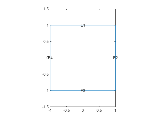
Specify the Dirichlet boundary condition for the left boundary.
applyBoundaryCondition(model,"dirichlet",Edge=4,u=0);Specify the zero Neumann boundary condition for the upper and lower boundary.
applyBoundaryCondition(model,"neumann",Edge=[1,3],g=0,q=0);Specify the generalized Neumann condition for the right boundary.
applyBoundaryCondition(model,"neumann",Edge=2,g=0,q=-3/4);The eigenvalue PDE coefficients for this problem are c = 1, a = 0, and d = 1. You can enter the eigenvalue range r as the vector [-Inf 10].
specifyCoefficients(model,m=0,d=1,c=1,a=0,f=0);
r = [-Inf,10];
Create a mesh and solve the problem.
generateMesh(model,Hmax=0.05);
results = solvepdeeig(model,r);
There are six eigenvalues smaller than 10 for this problem.
l = results.Eigenvalues
l = 5×1

   -0.4146
    2.0528
    4.8019
    7.2693
    9.4550
Plot the first and last eigenfunctions in the specified range.
u = results.Eigenvectors;
pdeplot(model,XYData=u(:,1));
axis equal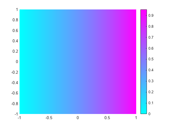
figure
pdeplot(model,XYData=u(:,length(l)));
axis equal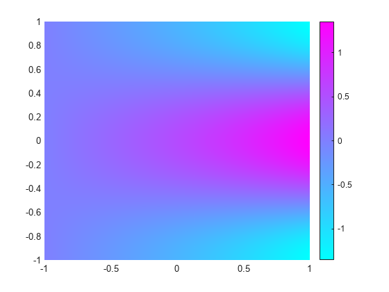
This problem is separable, meaning
The functions f and g are eigenfunctions in the x and y directions, respectively. In the x direction, the first eigenmode is a slowly increasing exponential function. The higher modes include sinusoids. In the y direction, the first eigenmode is a straight line (constant), the second is half a cosine, the third is a full cosine, the fourth is one and a half full cosines, etc. These eigenmodes in the y direction are associated with the eigenvalues
It is possible to trace the preceding eigenvalues in the eigenvalues of the solution. Looking at a plot of the first eigenmode, you can see that it is made up of the first eigenmodes in the x and y directions. The second eigenmode is made up of the first eigenmode in the x direction and the second eigenmode in the y direction.
Look at the difference between the first and the second eigenvalue compared to :
l(2) - l(1) - pi^2/4
ans =
1.6351e-07
Likewise, the fifth eigenmode is made up of the first eigenmode in the x direction and the third eigenmode in the y direction. As expected, l(5)-l(1) is approximately equal to :
l(5) - l(1) - pi^2
ans =
6.0246e-06
You can explore higher modes by increasing the search range to include eigenvalues greater than 10.