Scattering Problem: PDE Modeler App
This example shows how to solve a simple scattering problem, where you compute the waves reflected by a square object illuminated by incident waves that are coming from the left. This example uses the PDE Modeler app. For the programmatic workflow, see Scattering Problem.
For this problem, assume an infinite horizontal membrane subjected to small vertical displacements U. The membrane is fixed at the object boundary. The medium is homogeneous, and the phase velocity (propagation speed) of a wave, α, is constant. The wave equation is
The solution U is the sum of the incident wave V and the reflected wave R:
U = V + R
When the illumination is harmonic in time, you can compute the field by solving a single steady problem. Assume that the incident wave is a plane wave traveling in the –x direction:
The reflected wave can be decomposed into spatial and time components:
Now you can rewrite the wave equation as the Helmholtz equation for the spatial component of the reflected wave with the wave number k = ω/α:
–Δr – k2r = 0
The Dirichlet boundary condition for the boundary of the object is U = 0, or in terms of the incident and reflected waves, R = -V. For the time-harmonic solution and the incident wave traveling in the –x direction, you can write this boundary condition as follows:
The reflected wave R travels outward from the object. The condition at the outer computational boundary must allow waves to pass without reflection. Such conditions are usually called nonreflecting. As approaches infinity, R approximately satisfies the one-way wave equation
This equation considers only the waves moving in the positive ξ-direction. Here, ξ is the radial distance from the object. With the time-harmonic solution, this equation turns into the generalized Neumann boundary condition
To solve the scattering problem in the PDE Modeler app, follow these steps:
Open the PDE Modeler app by using the
pdeModelercommand.Set the x-axis limit to
[0.1 1.5]and the y-axis limit to[0 1]. To do this, select Options > Axes Limits and set the corresponding ranges.Display grid lines. To do this:
Select Options > Grid Spacing and clear the Auto checkboxes.
Enter X-axis linear spacing as
0.1:0.05:1.5and Y-axis linear spacing as0:0.05:1.Select Options > Grid.
Align new shapes to the grid lines by selecting Options > Snap.
Draw a square with sides of length 0.1 and a center in
[0.8 0.5]. To do this, first click the button. Then right-click the origin and drag to draw a square.
Right-clicking constrains the shape you draw so that it is a square rather than a rectangle.
If the square is not a perfect square, double-click it. In the resulting dialog box, specify
the exact location of the bottom left corner and the side length.
button. Then right-click the origin and drag to draw a square.
Right-clicking constrains the shape you draw so that it is a square rather than a rectangle.
If the square is not a perfect square, double-click it. In the resulting dialog box, specify
the exact location of the bottom left corner and the side length.Rotate the square by 45 degrees. To do this, select Draw > Rotate... and enter 45 in the resulting dialog box. The rotated square represents the illuminated object.
Draw a circle with a radius of 0.45 and a center in
[0.8 0.5]. To do this, first click the button. Then right-click the origin and drag to draw a circle.
Right-clicking constrains the shape you draw so that it is a circle rather than an ellipse.
If the circle is not a perfect unit circle, double-click it. In the resulting dialog box,
specify the exact center location and radius of the circle.
button. Then right-click the origin and drag to draw a circle.
Right-clicking constrains the shape you draw so that it is a circle rather than an ellipse.
If the circle is not a perfect unit circle, double-click it. In the resulting dialog box,
specify the exact center location and radius of the circle.Model the geometry by entering
C1-SQ1in the Set formula field.Check that the application mode is set to
Generic Scalar.Specify the boundary conditions. To do this, switch to the boundary mode by selecting Boundary > Boundary Mode. Use Shift+click to select several boundaries. Then select Boundary > Specify Boundary Conditions.
For the perimeter of the circle, the boundary condition is the Neumann boundary condition with
q = -ik, where the wave numberk = 60corresponds to a wavelength of about 0.1 units. Enterg = 0andq = -60*i.For the perimeter of the square, the boundary condition is the Dirichlet boundary condition:
In this problem, because the reflected wave travels in the –x direction, the boundary condition is r = –e–ikx. Enter
h = 1andr = -exp(-i*60*x).
Specify the coefficients by selecting PDE > PDE Specification or clicking the
 button on the toolbar. The Helmholtz equation is a wave
equation, but in Partial Differential Equation Toolbox™ you can treat it as an elliptic equation with
button on the toolbar. The Helmholtz equation is a wave
equation, but in Partial Differential Equation Toolbox™ you can treat it as an elliptic equation with a = -k2. Specifyc = 1,a = -3600, andf = 0.Initialize the mesh by selecting Mesh > Initialize Mesh.
For sufficient accuracy, you need about 10 finite elements per wavelength. The outer boundary must be located a few object diameters away from the object itself. Refine the mesh by selecting Mesh > Refine Mesh. Refine the mesh two more times to achieve the required resolution.
Solve the PDE by selecting Solve > Solve PDE or clicking the
 button on the toolbar.
The solution is complex. When plotting the solution, you get a warning message.
Plot the reflected waves. Change the colormap to
jetby selecting Plot > Parameters and then selectingjetfrom the Colormap drop-down menu.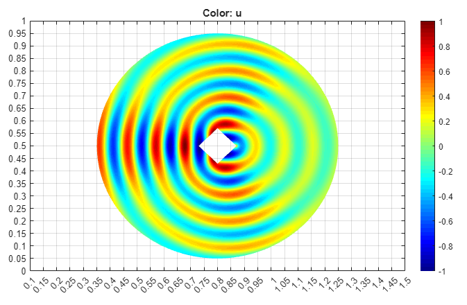
Animate the solution for the time-dependent wave equation. To do this:
Export the mesh data and the solution to the MATLAB® workspace by selecting Mesh > Export Mesh and Solve > Export Solution, respectively.
Enter the following commands in the MATLAB Command Window.
figure
maxu = max(abs(u));
m = 10;
for j = 1:m,
   uu = real(exp(-j*2*pi/10*sqrt(-1))*u);
   pdeplot(p,e,t,'XYData',uu,'ColorBar','off','Mesh','off');
   colormap(jet)
   caxis([-maxu maxu]);
   axis tight
   ax = gca;
   ax.DataAspectRatio = [1 1 1];
   axis off
   M(:,j) = getframe;
 end
movie(M);