Stress Concentration in Plate with Circular Hole
Perform a 2-D plane-stress elasticity analysis.
A thin rectangular plate under a uniaxial tension has a uniform stress distribution. Introducing a circular hole in the plate disturbs the uniform stress distribution near the hole, resulting in a significantly higher than average stress. Such a thin plate, subject to in-plane loading, can be analyzed as a 2-D plane-stress elasticity problem. In theory, if the plate is infinite, then the stress near the hole is three times higher than the average stress. For a rectangular plate of finite width, the stress concentration factor is a function of the ratio of hole diameter to the plate width. This example approximates the stress concentration factor using a plate of a finite width.
Create Geometry
The plate must be sufficiently long, so that the applied loads and boundary conditions are far from the circular hole. This condition ensures that a state of uniform tension prevails in the far field and, therefore, approximates an infinitely long plate. In this example the length of the plate is four times greater than its width. Specify the following geometric parameters of the problem.
radius = 20.0;
totalWidth = 50.0;
totalLength = 4*totalWidth;
Define the geometry description matrix (GDM) for the rectangle and circle.
R1 = [3 4 -totalLength  totalLength ...
           totalLength -totalLength ...
          -totalWidth -totalWidth totalWidth totalWidth]';
C1 = [1 0 0 radius 0 0 0 0 0 0]';
Define the combined GDM, name-space matrix, and set formula to construct decomposed geometry using decsg.
gdm = [R1 C1];
ns = char('R1','C1');
g = decsg(gdm,'R1 - C1',ns');
Plot the geometry with edge labels.
figure
pdegplot(g,EdgeLabel="on");
axis([-1.2*totalLength 1.2*totalLength -1.2*totalWidth 1.2*totalWidth])
title("Geometry with Edge Labels")

Plot the geometry with vertex labels.
figure
pdegplot(g,VertexLabels="on");
axis([-1.2*totalLength 1.2*totalLength -1.2*totalWidth 1.2*totalWidth])
title("Geometry with Vertex Labels")

Specify Parameters for Structural Analysis
Create an femodel object for static structural analysis and include the geometry into the model. By default, femodel assumes that a 2-D problem is a plane-stress problem.
model = femodel(AnalysisType="structuralStatic", ...
                Geometry=g);
Specify Young's modulus and Poisson's ratio.
model.MaterialProperties = ...
    materialProperties(YoungsModulus=200E3, ...
                       PoissonsRatio=0.25);
Apply the surface traction with a nonzero x-component on the right edge of the plate.
model.EdgeLoad(2) = edgeLoad(SurfaceTraction=[100;0]);
Restrain all rigid-body motions of the plate by specifying sufficient constraints. For static analysis, the constraints must also resist the motion induced by applied load. Set the x-component of displacement on the left edge (edge 4) to zero to resist the applied load.
model.EdgeBC(4) = edgeBC(XDisplacement=0);
Set the y-component of displacement at the bottom left corner (vertex 1) to zero to restraint the rigid body motion.
model.VertexBC(1) = vertexBC(YDisplacement=0);
Generate Mesh and Solve
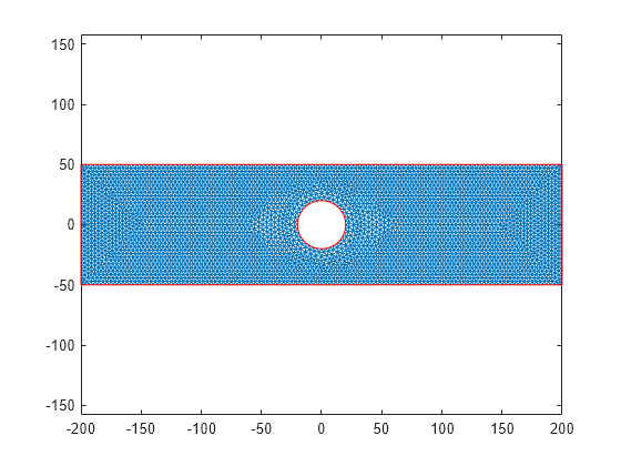
To capture the gradation in solution accurately, use a fine mesh. Generate the mesh, using Hmax to control the mesh size.
model = generateMesh(model,Hmax=radius/6);
Plot the mesh.
figure
pdemesh(model)

Solve the plane-stress elasticity model.
R = solve(model);
Plot Stress Contours
Plot the x-component of the normal stress distribution. The stress is equal to applied tension far away from the circular boundary. The maximum value of stress occurs near the circular boundary.
figure
pdeplot(R.Mesh,XYData=R.Stress.sxx, ...
        ColorMap="jet")
axis equal
title("Normal Stress Along x-Direction")

Interpolate Stress
To see the details of the stress variation near the circular boundary, first define a set of points on the boundary.
thetaHole = linspace(0,2*pi,200);
xr = radius*cos(thetaHole);
yr = radius*sin(thetaHole);
CircleCoordinates = [xr;yr];
Then interpolate stress values at these points by using interpolateStress. This function returns a structure array with its fields containing interpolated stress values.
stressHole = interpolateStress(R,CircleCoordinates);
Plot the normal direction stress versus angular position of the interpolation points.
figure
plot(thetaHole,stressHole.sxx)
xlabel("\theta")
ylabel("\sigma_{xx}")
title("Normal Stress Around Circular Boundary")

Solve the Same Problem Using Symmetric Model
The plate with a hole model has two axes of symmetry. Therefore, you can model a quarter of the geometry. The following model solves a quadrant of the full model with appropriate boundary conditions.
Create the geometry that represents one quadrant of the original model. You do not need to create additional edges to constrain the model properly.
R1 = [3 4 0 totalLength/2 totalLength/2 ...
      0 0 0 totalWidth totalWidth]';
C1 = [1 0 0 radius 0 0 0 0 0 0]';
gm = [R1 C1];
sf = 'R1-C1';
ns = char('R1','C1');
g = decsg(gm,sf,ns');
Plot the geometry displaying the edge labels.
figure
pdegplot(g,EdgeLabel="on");
axis equal
title("Symmetric Quadrant with Edge Labels")

Create an femodel object for static structural analysis and include the geometry into the model.
model = femodel(AnalysisType="structuralStatic",...
                Geometry=g);
Specify structural properties of the material.
model.MaterialProperties = ...
    materialProperties(YoungsModulus=200E3, ...
                       PoissonsRatio=0.25);
Apply surface traction on the edge 1.
model.EdgeLoad(1) = edgeLoad(SurfaceTraction=[100;0]);
Restrain all rigid-body motions of the plate by specifying sufficient constraints. For static analysis, the constraints must also resist the motion induced by applied load. Set the x-component of displacement on the left edge (edge 4) to zero to resist the applied load.
model.EdgeBC(4) = edgeBC(XDisplacement=0);
Set the y-component of displacement at the bottom edge (edge 3) to zero to restraint the rigid body motion.
model.EdgeBC(3) = edgeBC(YDisplacement=0);
Generate mesh and solve the symmetric plane-stress model.
model = generateMesh(model,Hmax=radius/6);
Rsym = solve(model);
Plot the x-component of the normal stress distribution. The results are identical to the first quadrant of the full model.
figure
pdeplot(Rsym.Mesh,XYData=Rsym.Stress.sxx, ...
                  ColorMap="jet");
axis equal
title("Normal Stress Along x-Direction for Symmetric Model")

