Main Content

phased.CustomFMWaveform

Custom FM pulse waveform

Since R2023a

Description

The phased.CustomFMWaveform System object™ lets you define a waveform with a user-defined frequency modulation (FM) and waveform envelope.

To create the waveform:

  1. Create the phased.CustomFMWaveform object and set its properties.

  2. Call the object with arguments, as if it were a function.

To learn more about how System objects work, see What Are System Objects?

Creation

Description

example

waveform = phased.CustomFMWaveform() creates a custom FM pulse waveform System object with linear frequency modulation and a rectangular envelope.

example

waveform = phased.CustomFMWaveform(Name=Value) sets additional properties using Name-Value arguments. You can specify additional name-value pair arguments in any order as (Neme1=Value1,…,NameN=ValueN).

Properties

expand all

Unless otherwise indicated, properties are nontunable, which means you cannot change their values after calling the object. Objects lock when you call them, and the release function unlocks them.

If a property is tunable, you can change its value at any time.

For more information on changing property values, see System Design in MATLAB Using System Objects.

Signal sample rate, specified as a positive scalar. The ratio of sample rate to pulse repetition frequency must be a positive integer, so the number of samples in each pulse must be an integer value. Units are in Hertz.

Example: 100e3

Data Types: double

Method to set pulse duration (pulse width), specified as 'Pulse width' or 'Duty cycle'. This property determines how you set the pulse duration.

  • When you set this property to 'Pulse width', set the pulse duration directly using the PulseWidth property.

  • When you set this property to 'Duty cycle', set the pulse duration from the values of the PRF and DutyCycle properties. The pulse width is equal to the value of the DutyCycle property divided by the value of the PRF property.

Data Types: char | string

Pulse time duration, specified as a positive scalar. The value must satisfy PulseWidth <= 1./PRF. Units are in seconds.

Dependencies

To enable this property, set the DurationSpecification property to 'Pulse width'.

Data Types: double

Pulse duty cycle, specified as a positive scalar in the range [0,1]. The pulse width is the value of the DutyCycle property divided by the value of the PRF property. This quantity is dimensionless.

Example: 0.75

Dependencies

To enable this property, set the DurationSpecification property to 'Duty cycle'.

Data Types: double

Pulse repetition frequency (PRF), specified as a scalar or a row vector. Units are in Hz. The pulse repetition interval (PRI) is the inverse of the pulse repetition frequency PRF value. The PRF must satisfy these restrictions:

  • The product of PRF and PulseWidth must be less than or equal to one. This condition requires that the pulse width is less than one PRI. For the phase-coded waveform, the pulse width is the product of the values of the ChipWidth and NumChips properties.

  • The ratio of SampleRate to PRF must be an integer. This condition requires that the number of samples in one PRI is an integer.

You can set the value of PRF using the PRF property settings alone or using property settings in conjunction with the prfidx input argument of the object.

  • When PRFSelectionInputPort is false, you set the PRF using the PRF properties alone. You can:

    • Implement a constant PRF by specifying the PRF property as a positive real-valued scalar.

    • Implement a staggered PRF by specifying the PRF property as a row vector with positive real-valued elements. Each call to the object uses successive elements of this vector as the PRF. Once the object reaches the last element of the vector, it continues the process cyclically with the first element of the vector.

  • When PRFSelectionInputPort is true, you can set the PRF value using the PRF property in conjunction with the prfidx input argument. You implement a selectable PRF by specifying the PRF property as a row vector with positive real-valued elements. When you execute the object, the object selects a PRF by using the index you specify in the prfidx input argument to index into the PRF vector.

In all cases, the number of output samples is fixed when you set the OutputFormat property to 'Samples'. When you use a varying PRF and also set the OutputFormat property to 'Pulses', the number of samples can vary.

Data Types: double

Enable PRF selection input, specified as false or true. When you set this property to true, you can pass an index argument to the object to select a predefined value from the PRF property vector. When you set this property to false, the object uses the PRF property to define the PRF sequence used in the simulation.

Data Types: logical

Waveform frequency modulation, specified as a length-M real-valued vector, function handle, or cell array.

  • If the FrequencyModulation property is a vector, it specifies samples of the instantaneous frequency at M points as [f1, f2, …, fM]. The waveform sweeps the specified frequencies such that for the kth pulse with start time tk and duration Tk, the instantaneous frequency at time

    tm=tk+(m1)Tk/(M1)

    is equal to fm where tktmtk + Tk and m = 1...M. The instantaneous frequencies between time tm and tm+1 are found by linearly interpolating between fm and fm+1. The resulting custom FM waveform is a piecewise linear FM (LFM) waveform consisting of M-1 LFM sections of equal duration.

  • If the FrequencyModulation property is a function handle, the function must have the following syntax: f = fmFcn(t) where f is the instantaneous frequency at time t. t is the time at which to compute the instantaneous frequency. The values in t are between 0 and the pulse width.

  • If the FrequencyModulation property is a cell array, then the first cell must be a function handle as specified above. The remaining entries in the cell array are the additional input arguments to the function, if any.

Data Types: double

Waveform envelope function, specified as 'Rectangular', 'Gaussian', 'Hamming', 'Chebyshev', 'Hann', 'Kaiser', 'Taylor', or 'Custom'.

When you set Envelope is set to 'Custom' must use the CustomEnvelope property to specify a custom envelope.

Example: 'Taylor'

Data Types: char | string

Sidelobe level for a Kaiser, Chebyshev, or Taylor window used as the waveform envelope, specified as a positive scalar. Units are in dB.

Dependencies

To enable this property, set the Envelope property to 'Kaiser', 'Chebyshev', or 'Taylor'.

Data Types: double

User-defined waveform envelope, specified as a function handle or cell array.

  • If CustomEnvelope is a function handle, the specified function uses the window length as input and generates appropriate window coefficients.

  • If CustomEnvelope is a cell array, then the first cell must be a function handle. The specified function takes the window length as the first input argument, with other additional input arguments if necessary, and generates appropriate window coefficients. The remaining entries in the cell array serve as additional input arguments to the function.

Example: {@chebwin,512,100}

Dependencies

To enable this property, set the Envelope property to 'Custom'.

Data Types: cell | function_handle

Source of frequency offset, specified as 'Property' or 'Input port'.

  • When you set this property to 'Property', the frequency offset is determined by the value of the FrequencyOffset property.

  • When you set this property to 'Input port', the frequency offset is determined by the input argument freqoffset when calling the object.

Example: 'Input port'

Data Types: char | string

Frequency offset, specified as a scalar. Units are in Hz.

Example: 150.0

Dependencies

To enable this property, set the FrequencyOffsetSource property to 'Property'.

Data Types: double

Format of output signal, specified as 'Pulses' or 'Samples'.

  • When you set the OutputFormat property to 'Pulses', the output of the object takes the form of multiple pulses specified by the value of the NumPulses property. The number of samples per pulse can vary if you change the PRF during the simulation.

  • When you set the OutputFormat property to 'Samples', the output of the object takes the form of multiple samples. In this case, the number of output signal samples is the value of the NumSamples property and is fixed.

Data Types: char | string

Number of samples in each output of the object, specified as a positive integer.

Dependencies

To enable this property, set the OutputFormat property to 'Samples'.

Data Types: double

Number of pulses in each output, specified as a positive integer.

Dependencies

To enable this property, set the OutputFormat property to 'Pulses'.

Data Types: double

Enable PRF output, specified as false or true. Set this property to true to output the PRF.

Dependencies

To enable this property, set the OutputFormat property to 'Pulses'.

Data Types: logical

Enable matched filter coefficients output, specified as false or true. Set this property to true to enable the object the output of the matched filter coefficients of the waveform used during the simulation.

Data Types: logical

Usage

Description

Y = waveform() returns samples of the custom nonlinear FM pulse in a column vector Y. Y can contain a certain number of pulses or a certain number of samples.

Y = waveform(prfidx) specifies the index of the PRF vector, prfidx. The object uses the index is used to identify the entries specified in the PRF property. To enable this syntax, set the PRFSelectionInputPort property to true.

Use this syntax for the cases where you need to dynamically select the transmitted pulse. In such situations, the PRF property includes a list of predetermined PRF values. During the simulation, based on PRF index input, the object selects one of the PRFs values for the PRF for the next transmission.

The transmission always finishes the current pulse before starting the next pulse. Therefore, when you set the OutputFormat property to 'Samples' and then specify the NumSamples property to be shorter than a pulse, the object can ignore the PRF index during a given simulation step if needs the entire output to finish the previously transmitted pulse.

Y = waveform(freqoffset) specifies the value of the frequency offset freqoffset. The offset generates the waveform with a frequency offset . Use this syntax when you need to update the transmit pulse frequency dynamically. To enable this syntax, set the FrequencyOffsetSource property to 'Input port'.

[Y,PRF] = waveform(___) also returns the current PRF. To enable this syntax, set the PRFOutputPort property to true and set the OutputFormat property to 'Pulses'.

[Y,coeff]= waveform() returns the matched filter coefficients coeff when you set the CoefficientsOutputPort property to true.

You can combine optional input and output arguments when you set their enabling properties are set. List optional inputs and outputs in the same order as the order of the enabling properties. For example,

[Y,PRF,coeff] = waveform(prfidx,freqoffset)

Input Arguments

expand all

Index of PRF, specified as a positive integer. The index identifies the entries in the PRF property. To enable this syntax, set the PRFSelectionInputPort property to true. Use this syntax when you need to dynamically select the transmit pulse. In such situations, the PRF property includes a list of predetermined values. During the simulation, based on the PRF index input, the object selects one of the PRFs is selected as the PRF for the next transmission.

Frequency offset, specified as a finite scalar. The object generates the waveform with a frequency offset. Use this syntax when you need to update the transmit pulse frequency dynamically.

Dependencies

To use this argument, set the FrequencyOffsetSource property to 'Input port'.

Data Types: double

Output Arguments

expand all

Pulse repetition frequency, returned as a scalar. When you set the PRFOutputPort property to true it returns the current PRF used by the system. Units are in Hz.

Dependencies

To enable this argument, set the PRFOutputPort property to true and set the OutputFormat to 'Pulses'.

Matched filter coefficients, returned as an NZ-by-1 complex-valued vector or an NZ-by-M complex-valued matrix.

  • If you set OutputFormat to 'Pulses' and NumPulses is 1, the object returns coeff as an NZ-length vector. NZ corresponds to the pulse width.

  • If you set OutputFormat to 'Pulses' with NumPulses greater than 1 or OutputFormat is 'Samples' and DurationSpecification is 'Pulse width', coeff is returned as an NZ-length vector. NZ corresponds to the pulse width.

  • If OutputFormat is set to 'Pulses' with NumPulses greater than 1 or OutputFormat is set to 'Samples' and DurationSpecification is set to 'Duty cycle' with only one unique PRF value, coeff is returned as an NZ-length vector. NZ corresponds to the pulse width.

  • If OutputFormat is 'Pulses' with NumPulses greater than 1 or OutputFormat is 'Samples' and DurationSpecification is 'Duty cycle', coeff is returned as an NZ-by-M matrix. NZ corresponds to the maximum pulse width and M corresponds to the number of unique PRFs.

Dependencies

To enable this argument, set the CoefficientsOutputPort property to true.

Data Types: double
Complex Number Support: Yes

Object Functions

To use an object function, specify the System object as the first input argument. For example, to release system resources of a System object named obj, use this syntax:

release(obj)

expand all

bandwidthWaveform bandwidth
getMatchedFilterMatched filter coefficients derived from waveform
plotPlot pulse waveform
stepRun System object algorithm
releaseRelease resources and allow changes to System object property values and input characteristics
resetReset internal states of System object

Examples

collapse all

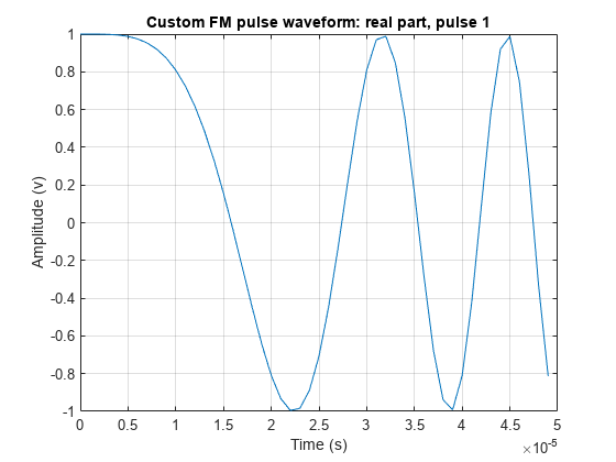
Create a custom FM waveform with the default frequency modulation and envelope function.

waveform = phased.CustomFMWaveform() 
waveform = 
  phased.CustomFMWaveform with properties:

                SampleRate: 1000000
     DurationSpecification: 'Pulse width'
                PulseWidth: 5.0000e-05
                       PRF: 10000
     PRFSelectionInputPort: false
       FrequencyModulation: [0 100000]
                  Envelope: 'Rectangular'
     FrequencyOffsetSource: 'Property'
           FrequencyOffset: 0
              OutputFormat: 'Pulses'
                 NumPulses: 1
             PRFOutputPort: false
    CoefficientsOutputPort: false

Display the real part of the waveform.

plot(waveform)

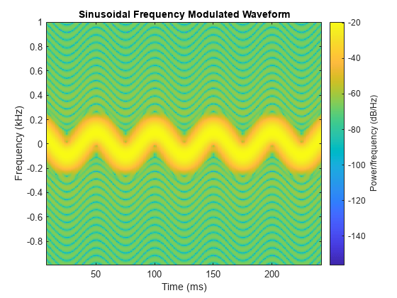
Create a sinusoidal frequency modulated waveform with a bandwidth of 200 Hz, a pulse width of 0.25 s, and a modulation frequency of 20 Hz.

BW = 200;
T = 0.25;
fm = 20;
fs = 10*BW;
freqfunc = @(t)(BW/2)*cos(2*pi*fm*t);
waveform = phased.CustomFMWaveform(SampleRate=fs, ...
    PulseWidth=T,FrequencyModulation=freqfunc,PRF=1/T);
wav = waveform();

Display the spectrogram of the waveform.

spectrogram(wav,32,30,512,fs,'yaxis','centered')
title('Sinusoidal Frequency Modulated Waveform')

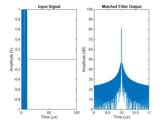
Create a nonlinear FM waveform derived from a power spectral density function shaped as a Taylor window with -35 dB sidelobes. The pulse bandwidth is 120 MHz and the pulse duration is10μsec. Generate matched filter coefficients and then apply a matched filter. Plot the resulting matched filter output to display the range sidelobe levels.

BW = 120e6;
T = 10e-6;
fs = 10*BW;

Generate 200 points of a waveform with instantaneous frequency values defined by a Taylor window. The window has -35 dB sidelobe levels.

w = taylorwin(200,4,-35);
freq = nlfmspec2freq(BW,w);
waveform = phased.CustomFMWaveform('SampleRate',fs, ...
    'PulseWidth',T,'FrequencyModulation',freq, ...
    'OutputFormat','Pulses','CoefficientsOutputPort',true);
disp(['Bandwidth = ',num2str(bandwidth(waveform)/1e6),' MHz'])
Bandwidth = 119.9644 MHz

Obtain the matched filter coefficients from the waveform.

[wav,coeff] = waveform();
mfilter = phased.MatchedFilter('CoefficientsSource','Input port');
mfout = mfilter(wav,coeff);

Plot input signal and matched filter output.

t = (0:numel(wav)-1)/fs;
figure
subplot(121)
plot(t*1e6,real(wav))
xlabel('Time (\mus)')
ylabel('Amplitude (V)')
title('Input Signal')

subplot(122)
plot(t*1e6,mag2db(abs(mfout)))
xlabel('Time (\mus)')
ylabel('Amplitude (dB)')
title('Matched Filter Output')
xlim([9 11])
ylim([0 100])

References

[1] Collins, T., and P. Atkins. "Nonlinear frequency modulation chirps for active sonar." IEE Proceedings-Radar, Sonar and Navigation 146.6 (1999): 312-316.

[2] Levanon, Nadav, and Eli Mozeson. Radar signals. John Wiley & Sons, 2004, pp. 92-93.

[3] Doerry, Armin Walter. "Generating nonlinear FM chirp waveforms for radar". No. SAND2006-5856. Sandia National Laboratories (SNL), Albuquerque, NM, and Livermore, CA (United States), 2006.

[4] Cook, C. E. "A class of nonlinear FM pulse compression signals." Proceedings of the IEEE 52.11 (1964): 1369-1371.

[5] Yang, J., and T. K. Sarkar. "Doppler‐invariant property of hyperbolic frequency modulated waveforms." Microwave and optical technology letters 48.6 (2006): 1174-1179.

[6] Melvin, William L., and James Scheer. Principles of modern radar: advanced techniques. SciTech Pub., 2013.

[7] Alphonse, Sebastian, and Geoffrey A. Williamson. "Evaluation of a class of NLFM radar signals." EURASIP Journal on Advances in Signal Processing 2019.1 (2019): 1-12.

Extended Capabilities

C/C++ Code Generation
Generate C and C++ code using MATLAB® Coder™.

Version History

Introduced in R2023a