FPGA-Based Range-Doppler Processing - Algorithm Design and HDL Code Generation
This example shows how to design a range-Doppler response that is ready for FPGA (field programmable gate array) implementation. The example matches the FPGA implementation to a corresponding behavioral model in Simulink® using the Phased Array System Toolbox™.
To verify the functional correctness of the hardware implementation model, the example compares the simulation output of that model with the results of the behavioral model. The term deployment here implies designing a model that is suitable for implementation on an FPGA. The model is deployment-ready and this condition is verified in the example. The hardware implementation is designed using fixed-point data types.
The Phased Array System Toolbox provides the floating-point behavioral model for the range-Doppler response through the phased.RangeDopplerResponse System object™. This behavioral model is used to verify the correctness of the implementation model.
Fixed-Point Designer™ provides data types and tools for developing fixed-point and single precision algorithms to optimize performance on an embedded hardware. Bit-true simulations can be performed to observe the impact of limited range and precision without implementing the design in hardware.
This example uses HDL Coder™ to generate HDL code from the developed Simulink model and verifies the HDL code using HDL Verifier™ tools. HDL Verifier is used to generate a cosimulation test bench model to verify the behavior of the automatically generated HDL code. The testbench uses ModelSim® for cosimulation of the generated HDL code.
Range-Doppler Response Algorithm
The phased.RangeDopplerResponse System object generates the range-Doppler Response using this algorithm.
Fast-time dimension: Filters the signal with a matched filter to generate the range response. The matched filter is an FIR filter with the coefficients set to the time-reverse replica of the transmitted signal.
Slow-time dimension: Computes the FFT to generate the Doppler response.
The input data is a matrix of M-by-N values, where M is the number of cells and N is the number of pulses. To calculate the range response, use an FIR filter across the rows (fast-time) and compute the FFT across the columns (slow-time).
Hardware Implementation Model
This example reuses the example input data and parameters from the phased.RangeDopplerResponse
Serialize and deserialize the signal by using the Serializer1D and Deserializer1D blocks, respectively. These blocks have input and output constraints for code generation, so set the FFT length to 64 and use a subset of the input data cube.
The implementation model uses a word length of 32 bits and a fraction length of 31 bits.
Open the Simulink model by using this command.
modelname = 'SLRangeDopplerHDL';
open_system(modelname);
% Ensure model is visible and not obstructed by scopes
scopes = find_system(modelname,'BlockType','Scope');
close_system(scopes);

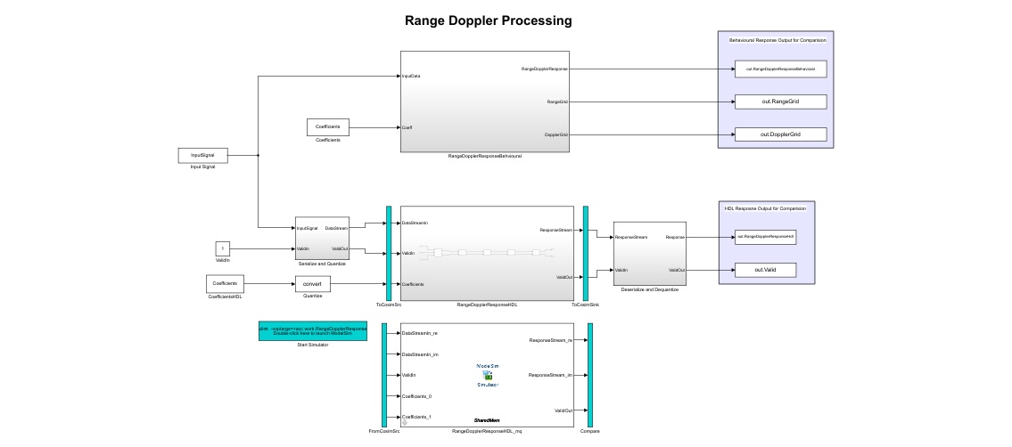
The Simulink model consists of two branches from the Input block. The top branch is the behavioral model with floating-point operations of the phased.RangeDopplerResponse System object. The bottom branch is the functionally equivalent implementation model using fixed-point data types, designed with blocks that support HDL code generation from the Simulink HDL Coder Library.
The input and coefficients are generated from the range-Doppler example data. The input is a M-by-N matrix, where M is the number of range cells (fast-time dimension) and N is the number of pulses (slow-time dimension). The output of the phased.RangeDopplerResponse object is a M-by-L matrix, where M is the number of range cells and L is the FFT length. Since the input and output of the implementation model have to be data streams, the input is serialized and quantized in the Serialize and Quantize subsystem and the output is deserialized to form a range-Doppler matrix map at the output in the Deserialize and Dequantize subsystem.
Preprocessing and Postprocessing Data
Open the Serialize and Quantize subsystem.
open_system([modelname '/Serialize and Quantize'])

The input data is zero-padded to accommodate the FIR filter latency by using the Matrix Concatenate block. The data is then serialized by a Serializer1D block used in cascade with the reshape and data-type convert (quantize to fixed-point) block.
open_system([modelname '/Deserialize and Dequantize'])

This subsystem uses a Deserializer1D block which uses the data-type convert and reshape blocks to convert the output stream to a range-Doppler map.
Matched Filtering - Range Processing Subsystem
open_system([modelname '/RangeDopplerResponseHDL/Matched Filtering - Range Processing'])

The input stream is processed with a Discrete FIR Filter block with the matching coefficients in the fast-time (row) dimension to get the range response. The block is suitable for hardware implementations and has a latency of seven cycles. The registers in the FIR filter have to be reset to an initial value of 0 after every row. This reset is performed by using a Boolean square wave implemented using a Counter and a Compare To Constant block.
Buffer & Transpose-Column
Open the Buffer & Transpose-Column subsystem.
open_system([modelname '/RangeDopplerResponseHDL/Buffer & Transpose - Column'])

The range-processed data is deserialized using cascaded Deserializer1D blocks and is converted to matrix format with a reshape block. This data is now zero padded and transposed for computing the FFT across the slow-time (column) dimension. The range-processed and transposed data is now serialized again for FFT computation (Doppler processing).
FFT-Doppler Processing
Open the FFT-Doppler Processing subsystem.
open_system([modelname '/RangeDopplerResponseHDL/FFT - Doppler Processing'])

The FFT of the streamed (across column) data is calculated using an FFT block which has a latency of 173 cycles. A streaming radix 2^2 architecture is used with an FFT length of 64.
Buffer-FFT Shift
Open the Buffer-FFT Shift subsystem.
open_system([modelname '/RangeDopplerResponseHDL/Buffer - FFT Shift'])

The Doppler-processed serial data is deserialized using Deserialized1D blocks and transposed. The FFT-processed data needs to be rearranged to have a zero-centric spectrum data, which is emulated by using a combination of selector blocks and a matrix concatenate.
Serialize Output
Open the Serialize Output subsystem.
open_system([modelname '/RangeDopplerResponseHDL/Serialize Output'])

The range-Doppler map data after processing is in the form of a matrix, which is then serialized using a Reshape and a Serializer1D block for the output stream.
Compare of Implementation Model and Behavioral Model Results
Simulate the model by clicking the Play button or by using the sim command.
out = sim(modelname);
To verify the functional correctness of the implementation model, subtract the response matrix of the behavioral model from the response matrix of the implementation model and check that the difference (error) is close to zero (or, within the quantization in the implementation model).
Export the response data from Simulink to the MATLAB® workspace, in the array format. Subtract the behavioral response vector from the implementation model response, reshape the error matrix into a 1-D array, and plot the error with the element index in the x-axis and error in the y-axis. Use the imagesc function to display the range-Doppler map. Use the following script to plot the response and error.
% Uncomment the following lines of code to visualize the response
% Behavioral Output
behavioralResponse = out.RangeDopplerResponseBehavioral(:,:,1);  % Response from To Workspace Block
behavioralResponsedB = mag2db(abs(behavioralResponse));          % Convert to dB
rangeGrid = out.RangeGrid(:,1,1);                                % Range Grid
dopplerGrid = out.DopplerGrid(:,1,1);                            % Doppler Grid
% Visualize the range-Doppler (Behavioral) map
f1 = figure(1);                                                  % Figure handle
f1.Name = 'Behavioral';                                          % Figure Name
fax1 = axes;                                                     % Axis Handle
imagesc(fax1,dopplerGrid,rangeGrid,behavioralResponsedB)
xlabel(fax1,'Doppler');
ylabel(fax1,'Range')
title(fax1,'Behavioral Response')
% HDL Output
idx = find(out.Valid);                                           % Search for valid output
HdlResponse = out.RangeDopplerResponseHdl(:,:,idx(1));           % Response from To Workspace Block
HdlResponsedB = mag2db(abs(HdlResponse));                        % Convert to dB
% Visualize the range-Doppler (HDL) map
f2 = figure(2);                                                  % Figure handle
f2.Name = 'HDL';                                                 % Figure Name
fax2 = axes;                                                     % Axis handle
imagesc(fax2,dopplerGrid,rangeGrid,HdlResponsedB);               % Use behavioral output of range and doppler grid
xlabel(fax2,'Doppler')
ylabel(fax2,'Range')
title(fax2,'HDL Response')
% Error
% Subtract the Behavioral Response from the HDL response
errorMatrix = abs(HdlResponse - behavioralResponse);             % Matrix Subtract
% Convert the error matrix into a row vector which can be visualised on a 2D axis
errorStream = reshape(errorMatrix,1,[]); % Convert error matrix to 1D, row wise
% Find the index and the maximum error between HDL and behavioral results
Ymax = max(errorStream);                                         % Find Maximum Error
Xmax = find(errorStream == Ymax);                                % Find index of maximum error
% Plot the error on a 2D plot and annotate the maximum error
% between HDL and behavioral response.
f3 = figure(3);                                                  % Figure handle
f3.Name = 'Error';                                               % Figure Name
fax3 = axes;                                                     % Axis handle
plot(fax3,errorStream)                                           % Plot
ylabel(fax3,'Error');
xlabel(fax3,'Data Point Index')
title(fax3,'Error between Behavioral and HDL Model');
textstr = strcat('     ErrorMax = ',num2str(Ymax));
text(fax3,Xmax,Ymax,textstr);
The figures show the range-Doppler map and the error between the behavioral and implementation models.


Code Generation and Verification
This section covers the procedure to generate HDL code for the range-Doppler response implementation model and verifying the functional correctness. The behavioral model provides the reference values to ensure that the output from HDL model is within tolerance limits. Based on the Simulink model setup described in the earlier sections, the implementation model is designed using fixed-point arithmetic blocks that support HDL code generation. Alternatively, if you start with a new model, you can run the hdlsetup function to configure the Simulink model for HDL code generation. To configure the Simulink model for test bench creation, open Model Settings, select Test Bench under HDL Code Generation in the left panel, and check HDL test bench and Cosimulation model in the Test Bench Generation Output properties group.
Model Settings
After the fixed-point implementation is verified and the implementation model produces the same results as your floating-point behavioral model, you can generate HDL code and test bench. For code generation and test bench, set these parameters in Model Settings under HDL Code Generation:
Target: Xilinx Vivado synthesis tool; Virtex7 family; Device xc7vx485t; package ffg1761, speed -1; and target frequency of 300 MHz.
Optimization: Clear all optimizations
Global Settings: Set the Reset type to Asynchronous.
Test Bench: Select HDL test bench and Cosimulation model
HDL Code Verification Using Cosimulation
After the model is set up, use the HDL Workflow Advisor to generate the HDL code using the HDL Coder tools, and generate a cosimulation test bench to test the model using HDL Verifier. To start the HDL Workflow Advisor, right-click on the RangeDopplerResponseHDL subsystem, then click HDL Code and HDL Workflow Advisor in the menu. Alternatively, you can use these commands to generate HDL code and test bench.
makehdl([modelname '/RangeDopplerResponseHDL']);   % Generate HDL code
makehdltb([modelname '/RangeDopplerResponseHDL']); % Generate Cosimulation test bench
After generating HDL code and the test bench, a new Simulink model named gm_SLRangeDopplerHDL_mq that contains a ModelSim® Cosimulation block is created in your working directory. This figure shows the generated model.
To open the test bench model use these commands.
modelname = ['gm_',modelname,'_mq'];
open_system(modelname);
Open ModelSim and run the cosimulation model to display the simulation results. You can click the Play button to run the test bench, or you can run it via command window using the following command.
sim(modelname);
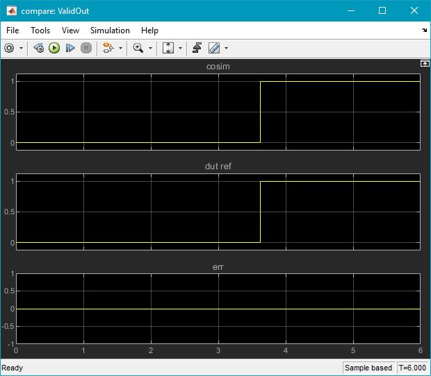
The Simulink test bench model configures QuestaSim® with the signal from the HDL model and Time Scope in Simulink.
The test bench scopes shows the output of the complex-valued response vector from the implementation model and the cosimulation output as well as the error between the two outputs.


Fixed-Point Word Length (Precision) and Resource Utilization Tradeoffs
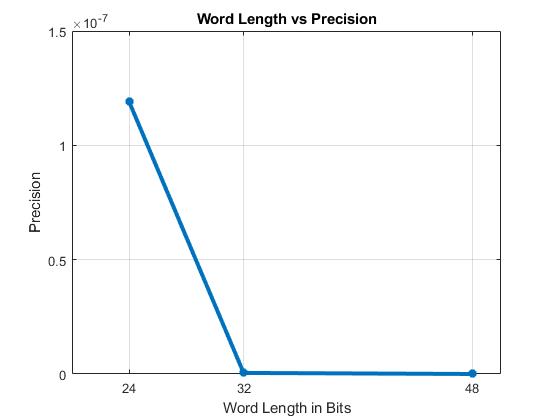
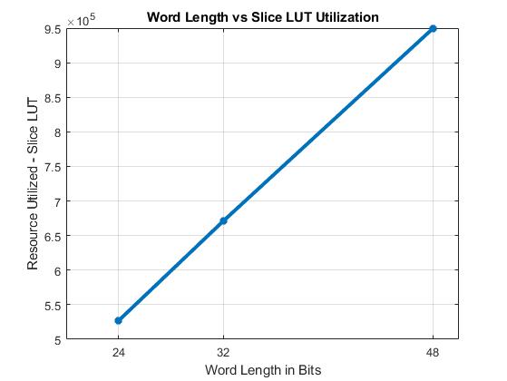
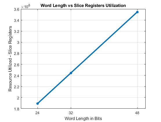
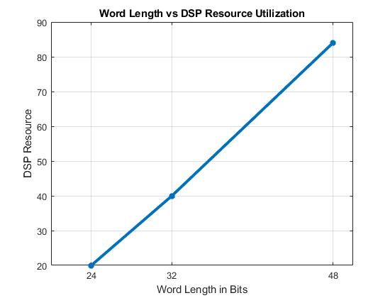
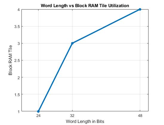
This example uses a word length of 32 bits and a fraction length of 31 bits for design, simulation, and implementation. There are tradeoffs associated with increasing the data precision with respect to resource utilization.
This figure shows the precision with respect to the word length.
The next figure shows the slice LUT utilization with respect to the word length.
The next figure shows the slice registers utilization with respect to the word length.
The next figure shows the DSP block utilization with respect to the word length.
The next figure shows the block RAM tile utilization with respect to the word length.
Summary
This example demonstrated a workflow for designing a Simulink model for a hardware-compatible range-Doppler response block, and verifying the results with equivalent behavioral code from the Phased Array System Toolbox. The example also shows how to generate HDL code for a fixed-point implementation and verifying the generated code in Simulink for functional correctness. This example showed how to set up and launch ModelSim to cosimulate the HDL code and compare its output to the output generated by the HDL implementation model.
