Power-Only Far-Field Calibration of Phased Arrays

R2026b

Since R2026b

Calibration of phased array antennas is critical to ensure that these systems meet their performance requirements when fielded in the real world. There are many approaches for calibrating antenna arrays. The approach is often limited by the information that is available when calibrating antenna arrays.

A common constraint during phased array calibration is that you only have access to the total power transmitted or received at some probing angle. In this case, you cannot measure signal powers on individual channels within the antenna array and you have no access to phase information.

This constraint arises when you are measuring total transmit power at a single probe location or are measuring total receive power at the output of a receive beamformer that combines signals at each antenna element into a single channel. This example discusses techniques that can be used to calibrate antenna arrays under this constraint.

Introduction

In this example we will implement a few common power only phased array calibration techniques. These calibration techniques relate only to far field array calibration. The performance of these methods will be compared by running Monte Carlo simulations across operating parameters such as signal-to-noise ratio (SNR) of the measurement setup and number of antenna elements. We will compare calibration error statistics as well as number of measurements required to determine the trade-offs that exist when selecting a power only calibration technique.

Power Only Array Calibration Overview

In power only calibration, the amplitude and phase of each element in an array are calibrated by varying the phase on individual channels within the array and measuring the combined power. A typical test setup is demonstrated below:

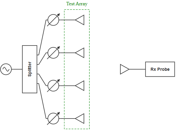
In this setup, the phase on each transmit channel is varied and the power is measured by a receive probe.

All of the power only calibration methods described in this example rely on varying the phase of a single element within an array while keeping the phase of all other elements constant. The diagram below demonstrates this calibration concept.

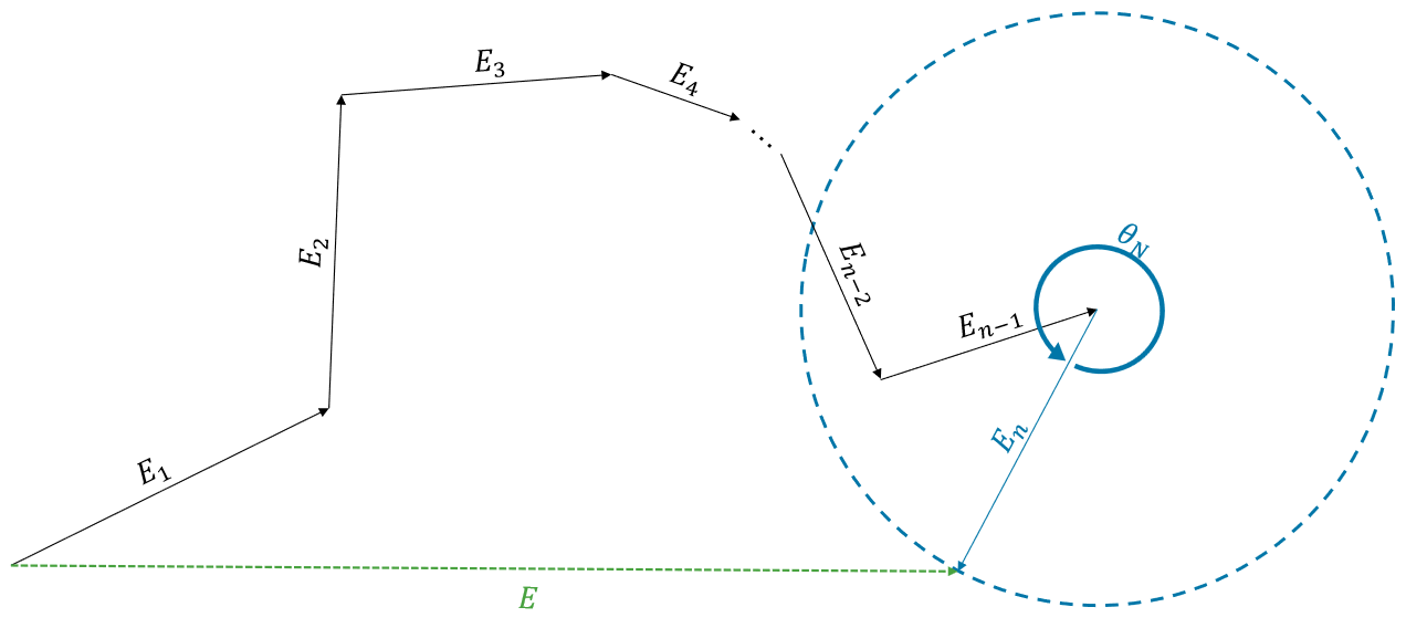
The contribution of each individual element vector to the full composite field vector is denoted by the complex number $E_i$, where i is the element index - summing together each of these contributions gives the full composite field vector $E$. In power only calibration we do not have access to the individual element contributions or even the amplitude and phase of the composite field vector - we only have access to power measurements which are ${\left|E\right|}^2$, where $\left|E\right|$ is the magnitude of the composite field vector.

As the phase of the test element vector $E_n$ changes, ${\left|E\right|}^2$ varies sinusoidally as shown in the following graph.

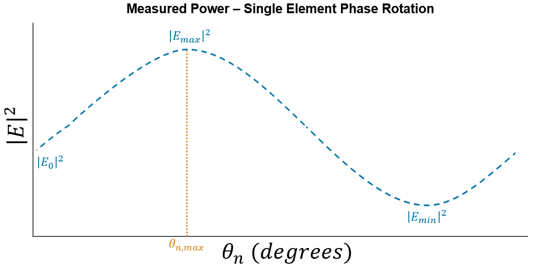
In power only calibration the goal is to measure the relative phase and amplitude in each channel of the antenna array. It is important to choose a common reference point against which to compare the phase and amplitude of each antenna element. For most algorithms, the initial state of the composite field vector $E_0$ is chosen.

Methods Discussed In This Example

Three popular power only calibration methods are discussed in this example. The algorithms are introduced in this section and are later discussed in more detail.

• Rotating Element Electric Field Vector (REV): This is the classical power only calibration technique. The composite field vector is measured at many phase shifts for each antenna element, and calibration values are determined based on the sinusoidal nature of the power measurements [1][2].

• Fast Method: This approach generates calibration weights with very few measurement points, making it very fast at the expense of some accuracy [3].

• Grouped REV Method: This approach measures the power variation when shifting the phase of groups of elements instead of a single element. This approach proves effective for large arrays [4].

Calibration Ambiguity

Many power only calibration methods require different equations for calculating phase and amplitude offsets of individual channels depending on whether the magnitude of the individual element field vector is less than or greater than the magnitude of the composite field vector minus the individual element field vector.

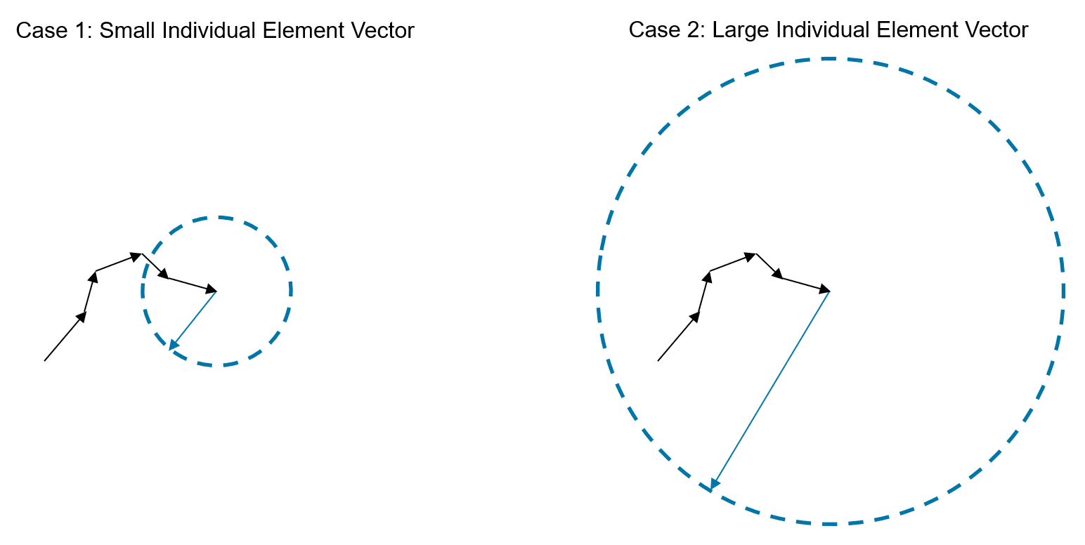
When only power level measurements are available, it can be difficult to distinguish between these two cases and always requires some extra data collection. It is oftentimes valid to assume that case 1 is correct, but this ambiguity may have to be accounted for in the real world.

Limitations

The power only calibration approaches discussed in this example only consider phase and amplitude calibration at a single observation angle. There is therefore an inherent assumption that the calibration errors are independent of angle, which is a simplification of reality. Depending on the nature of the array being used and the accuracy requirements of the calibration, this may be a good assumption, or calibration measurements may be required at a large number of observation angles.

Calibration Algorithm Implementations

In this section we discuss the implementation of each calibration algorithm.

Simulation

In order to demonstrate each calibration algorithm we set up a simple simulation of a 32-element uniform linear array transmitting a 10 GHz tone and an isotropic receive probe is placed in the far field at boresight to measure the combined signal. Phase and amplitude calibration errors are set using the Taper property of the transmit array.

% Set random number generator for reproducibility
rng('default');

% Create transmit array
fc = 10e9;
lambda = freq2wavelen(fc);
spacing = lambda/2;
numElements = 32;
txArray = phased.ULA(NumElements=numElements, ElementSpacing=spacing);
radiator = phased.Radiator(Sensor=txArray,OperatingFrequency=fc,WeightsInputPort=true);

% Create some calibration errors and set them on the array
ampErr = 1+0.2*rand(1,numElements);
phaseErr = randn(1,numElements)*pi/4;
calErr = ampErr.*exp(1i*phaseErr);
txArray.Taper = calErr;

% Create a constant amplitude calibration signal
nSamples = 100;
calSig = ones(nSamples,1);

% Create probe antenna
rxAntenna = phased.IsotropicAntennaElement;
collector = phased.Collector(Sensor=rxAntenna,OperatingFrequency=fc);

% Create receiver - this is modeled as white gaussian noise followed by a power
% detector
awgnSnr = 100;
noiseFcn = @(x)awgn(x,awgnSnr);
powFcn = @(x)abs(x).^2;
behaviorFcn = @(x)powFcn(noiseFcn(x));
receiver = phased.Receiver(Configuration="Cascade",Cascade={phased.CustomCascadeComponent(BehaviorFcn=behaviorFcn)});

% Assume the receiver is placed in the far field of the transmitter at
% boresight
txAng = [0;0];
rxAng = [180;0];

With the simulation setup, we can show how the power measurements vary as a function of phase-shift angle for the first element.

nTest = 100;
testPhaseShifts = helperGetEvenlySpacedPhases(nTest);
power = zeros(1,nTest);
eut = 1;
for iPhase = 1:nTest
    % Create the steering weights with the desired phase shift on the
    % element under test
    weights = ones(numElements,1);
    phaseShift = testPhaseShifts(iPhase);
    weights(eut) = exp(1i*phaseShift/360*2*pi);

    % Simulate signal transmission and reception
    txSig = radiator(calSig,txAng,weights);
    collectSig = collector(txSig,rxAng);
    sigPower = receiver(collectSig);

    % Record the mean output power
    power(iPhase) = mean(sigPower);
end

% Plot the measured power as phase shift of the first element changes
helperDisplayPowerSinusoid(testPhaseShifts,power,eut);

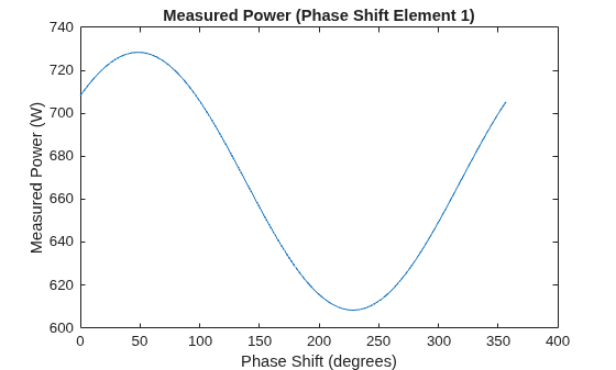
We observe the expected sinusoidal shape described in the introduction. We can now investigate the implementation of the methods of interest using this simulation setup.

Rotating Element Electric Field Vector (REV) Method

In this section we implement the standard REV method from [1].

REV Overview

The goal of this method is to determine the amplitude and phase shift of a single element vector with respect to the original composite field vector:

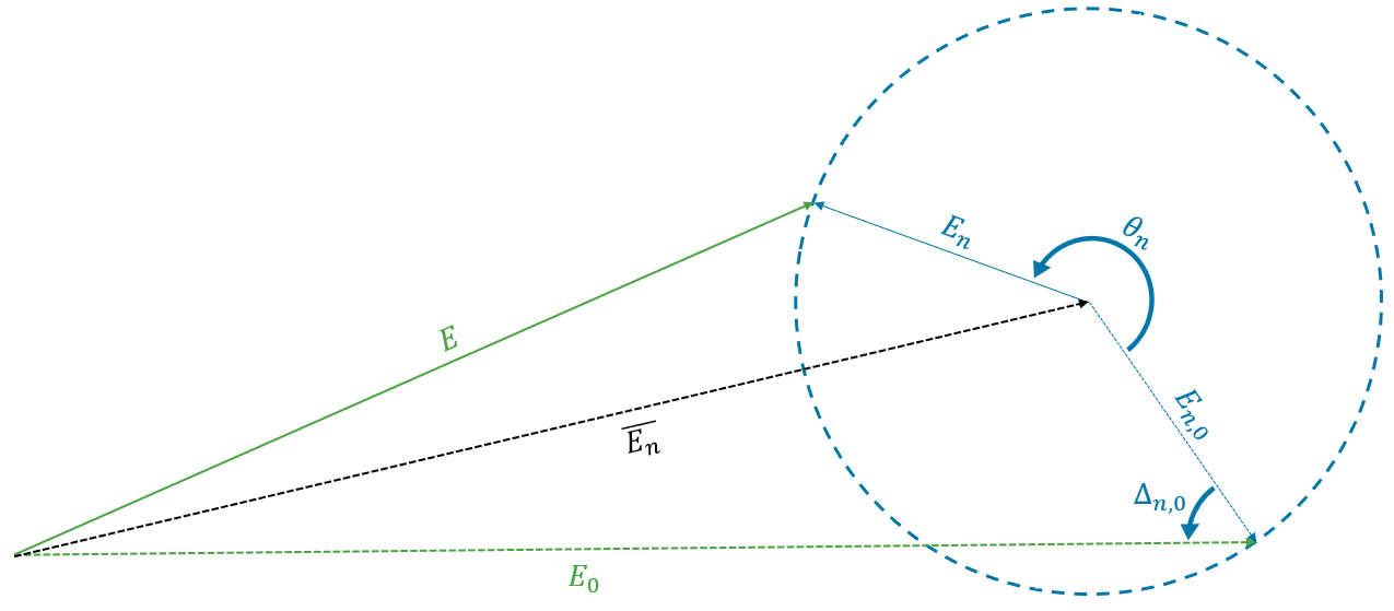
In this diagram, $\underset{}{\overset{‾}{E_n}}$ is the composite field vector without the element under test, $E_0$ is the composite field vector with no phase shifts applied and $E_{n,0}$ is the original field vector for the element under test. Ultimately, the calibration values that we are seeking are:

• $\frac{\left|E_n\right|}{\left|E_0\right|}$: the magnitude of the element vector with respect to the original composite vector.

• ${\Delta }_{n,0}$: the phase of the original element vector with respect to the original composite vector.

The relationship between the measured signal and the signals without any additional calibration phase shifts are given by the following equation:

$$E=E_0-E_{n,0}+E_n$$

By formulating the relative power of $E_n$ with respect to $E_0$, the authors of the original REV formulation determine the equations for the calibration values based on this signal equation.

It turns out that there are two solutions depending on the ambiguity described in the introduction.

For the case where $\left|{\underset{}{\overset{‾}{E}}}_n\right|>\left|E_n\right|$, the equations for the calibration values are:

$$\frac{\left|E_n\right|}{\left|E_0\right|}=\frac{\Gamma }{\sqrt{1+2\Gamma \cos \left({\theta }_{n,\max }\right)+{\Gamma }^2}}$$

$${\Delta }_{n,0}={\tan }^{-1}\left(\frac{\sin \left({\theta }_{n,\max }\right)}{\cos \left({\theta }_{n,\max }\right)+\Gamma }\right)$$

For the case where $\left|{\underset{}{\overset{‾}{E}}}_n\right|<\left|E_n\right|$, a different set of equations are required:

$$\frac{\left|E_n\right|}{\left|E_0\right|}=\frac{1}{\sqrt{1+2\Gamma \cos \left({\theta }_{n,\max }\right)+{\Gamma }^2}}$$

$${\Delta }_{n,0}={\tan }^{-1}\left(\frac{\sin \left({\theta }_{n,\max }\right)}{\cos \left({\theta }_{n,\max }\right)+\frac{1}{\Gamma }}\right)$$

Where:

$$\Gamma =\frac{\left|E_{\max }\right|-\left|E_{\min }\right|}{\left|E_{\max }\right|+\left|E_{\min }\right|}$$

For a full derivation of these equations, see [1]. There are various methods that can be used to determine which is the correct case, however in this section we will assume case 1 is correct and provide one method for determining which case is correct when discussing a related calibration method.

There are three unknowns in each of these sets of equations that we need:

• ${\theta }_{n,\max }$: The phase shift applied to the element under test that results in the maximum received power.

• $\left|E_{\max }\right|$: The maximum received amplitude.

• $\left|E_{\min }\right|$: The minimum received amplitude.

The goal of REV is to measure these terms and use them to generate calibration values for each element in an antenna array.

The following function implements the REV algorithm for a single element.

function calWeight = helperRev(phaseShifts,measuredPower,ambiguityCase)
    % Get magnitude from power
    e = sqrt(measuredPower);

    % Calculate Emax, Emin, and max angle
    [eMax,maxIdx] = max(e);
    eMin = min(e);
    maxPhase = phaseShifts(maxIdx);

    % Output the calibration weights based on Emax, Emin, max angle, and
    % whether this is case 1 or case 2.
    calWeight = helperApplyRevEqns(eMax,eMin,maxPhase,ambiguityCase);
end

function calWeight = helperApplyRevEqns(eMax,eMin,maxPhase,ambiguityCase)
    % Apply REV algorithm case 1 or case 2.
    if ambiguityCase == 1
        [calMag,calPhase] = helperRevCase1(eMax,eMin,-maxPhase);
    else
        [calMag,calPhase] = helperRevCase2(eMax,eMin,-maxPhase);
    end

    % Save cal weights
    calWeight = calMag*exp(1i*calPhase);
end

function [calMag,calPhase] = helperRevCase1(eMax,eMin,maxPhase)
    % Case 1 REV equations
    gamma = helperRevGamma(eMax,eMin);
    denominator = helperRevDenominator(gamma,maxPhase);
    calMag = gamma/denominator;
    calPhase = atan(sind(maxPhase)/(cosd(maxPhase)+gamma));
end

function [calMag,calPhase] = helperRevCase2(eMax,eMin,maxPhase)
    % Case 2 REV equations
    gamma = helperRevGamma(eMax,eMin);
    denominator = helperRevDenominator(gamma,maxPhase);
    calMag = 1/denominator;
    calPhase = atan(sind(maxPhase)/(cosd(maxPhase)+1/gamma));
end

function gamma = helperRevGamma(eMax,eMin)
    % Calculate gamma value
    gamma = (eMax-eMin)/(eMax+eMin);
end

function denominator = helperRevDenominator(gamma,maxPhase)
    % Calculate denominator of magnitude in the REV equation
    denominator = sqrt(1+2*gamma*cosd(maxPhase)+gamma^2);
end

REV Demonstration

In the classic implementation of the REV method, every phase shift setting for every element is stepped through. The number of phase shift settings depend on the number of phase shift bits. For this demonstration we assume that there are 8 bits.

nBits = 8;
nps = 2^nBits;
testPhaseShifts = helperGetEvenlySpacedPhases(nps);

We use the signal propagation model described in the simulation section to record the measured power deviation across phase shifts for each element.

estCalWeights = ones(1,numElements);
for iElement = 1:numElements
    % Record the power measured for each element
    power = zeros(nps,1);

    % Measure power at each phase shift
    for ips = 1:nps
        ps = testPhaseShifts(ips);
        testWeights = ones(numElements,1);
        testWeights(iElement) = exp(1i*deg2rad(ps));
        power(ips) = helperMeasurePower(calSig,txAng,rxAng,radiator,collector,receiver,testWeights);
    end

    % Apply REV algorithm (assumes case 1 by default).
    estCalWeights(iElement) = helperRev(testPhaseShifts,power,1);
end

After estimating the calibration weights, we can compare with the true calibration weights when normalized against the composite field vector.

fv = sum(calErr);
trueCalWeights = calErr / fv;
helperShowCalibrationError(estCalWeights,trueCalWeights);

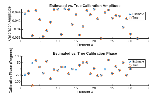
REV gives a good estimate of the true calibration weights under these conditions.

Reducing Measurement Points: Sinusoidal Curve Fit

The classic REV method uses $2^B$ measurement points for each element in the array, where B = number of phase shift bits. The measurement value when phase shift set to 0 is the same for each element, so the required number of measurements for classic REV is $N*\left(2^B-1\right)+1$ where N is the number of antenna elements.

There are a number of proposed methods for reducing the required number of measurement points when performing power only calibration. One popular approach is to simply take fewer measurements and fit a sinusoid to the measurement points. The frequency of the measured sinusoid is known, so technically only 3 measurement points are required to estimate the amplitude, phase, and offset of the sinusoid. In practice, more measurement points are required - in [3] it is suggested that at least 8 different phase shifts per element should be measured, including 0 degrees, so that the total number of measurements are 7N+1.

The following helper function demonstrates how this modification would work.

function calWeight = helperRevBestFit(phaseShifts,measuredPower,ambiguityCase)
    % Get the max value, min value, and phase where max occurs
    [eMax,eMin,maxPhase] = helperSinusoidFit(phaseShifts,measuredPower);

    % Output the calibration weights based on Emax, Emin, max angle, and
    % whether this is case 1 or case 2.
    calWeight = helperApplyRevEqns(eMax,eMin,maxPhase,ambiguityCase);
end

function [eMax,eMin,maxPhase] = helperSinusoidFit(phaseShifts,measuredPower)
    % Use linear regression to fit Asin(x)+Bcos(x)+C
    H = [sind(phaseShifts(:)), cosd(phaseShifts(:)), ones(size(phaseShifts(:)))];    
    theta = H \ measuredPower(:);
    A = theta(1);
    B = theta(2);
    C = theta(3);
    
    % Get eMax and eMin
    amp = hypot(A,B);
    eMax = sqrt(max(C+amp, 0));
    eMin = sqrt(max(C-amp, 0));

    % Get maxPhase, which occurs when A*cos(x) = B*cos(x)
    xpeak1 = rad2deg(atan2(A,B));
    v1 = A*sind(xpeak1)+B*cosd(xpeak1)+C;
    xpeak2 = wrapTo360(xpeak1+180);
    v2 = A*sind(xpeak2)+B*cosd(xpeak2)+C;
    if v1 > v2
        maxPhase = xpeak1;
    else
        maxPhase = xpeak2;
    end
end

Using this approach, we reduce the number of measurement points to 8 per element.

nPoints = 8;
testPhaseShifts = helperGetEvenlySpacedPhases(nPoints);
estCalWeights = ones(1,numElements);
for iElement = 1:numElements
    % Record the power measured for each element
    power = zeros(nPoints,1);

    % Measure power at each phase shift
    for ips = 1:nPoints
        ps = testPhaseShifts(ips);
        testWeights = ones(numElements,1);
        testWeights(iElement) = exp(1i*deg2rad(ps));
        power(ips) = helperMeasurePower(calSig,txAng,rxAng,radiator,collector,receiver,testWeights);
    end

    % Apply REV algorithm using sinusoid fit (assumes case 1 by default).
    estCalWeights(iElement) = helperRevBestFit(testPhaseShifts,power,1);
end

Once again, we compare with the true calibration weights.

helperShowCalibrationError(estCalWeights,trueCalWeights);

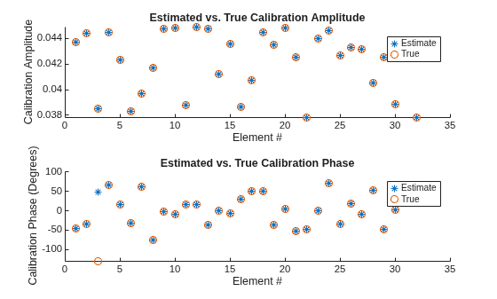
These results still closely approximate the true calibration values despite substantially fewer measurements.

Fast Calibration Method

The method discussed in [3] requires an even smaller number of measurement points than using a sinusoidal approximation in REV. Instead of formulating the calibration problem geometrically by determining the shape of a sinusoid, a system of linear equations is set up by using the inner product of the signals as intermediate parameters.

In this approach, only 3 measurement points are required for each antenna element at phase shifts of $0,\frac{\pi }{2},$and $\pi$radians. Because the 0 phase offset power measurement is the same for each element, the total number of measurements required for the full array is only $2N+1$ using this method.

The core equations in this approach are developed by stating the power received in terms of the inner product of the sum of $\underset{}{\overset{‾}{E_n}}+E_n$:

$$P_0=\left(\left|\underset{}{\overset{‾}{E_n}}\right|e^{j\angle \underset{}{\overset{‾}{E_n}}}+\left|E_n\right|e^{j\angle E_n}\right){\left(\left|\underset{}{\overset{‾}{E_n}}\right|e^{j\angle \underset{}{\overset{‾}{E_n}}}+\left|E_n\right|e^{j\angle E_n}\right)}^{*}$$

$$P_{\frac{\pi }{2}}=\left(\left|\underset{}{\overset{‾}{E_n}}\right|e^{j\angle \underset{}{\overset{‾}{E_n}}}+\left|E_n\right|e^{j\left(\angle E_n+\frac{\pi }{2}\right)}\right){\left(\left|\underset{}{\overset{‾}{E_n}}\right|e^{j\angle \underset{}{\overset{‾}{E_n}}}+\left|E_n\right|e^{j\left(\angle E_n+\frac{\pi }{2}\right)}\right)}^{*}$$

$$P_{\pi }=\left(\left|\underset{}{\overset{‾}{E_n}}\right|e^{j\angle \underset{}{\overset{‾}{E_n}}}+\left|E_n\right|e^{j\left(\angle E_n+\pi \right)}\right){\left(\left|\underset{}{\overset{‾}{E_n}}\right|e^{j\angle \underset{}{\overset{‾}{E_n}}}+\left|E_n\right|e^{j\left(\angle E_n+\pi \right)}\right)}^{*}$$

These equations can be rearranged to give a system of linear equations:

$$\left[\begin{array}{ccc}1& 1& 1\\ 1& -j& j\\ 1& -1& -1\end{array}\right]\left[\begin{array}{c}\left({\left|{\underset{}{\overset{‾}{E}}}_n\right|}^2+{\left|E_n\right|}^2\right)\\ \left|{\underset{}{\overset{‾}{E}}}_n\right|\left|E_n\right|e^{j\left(\angle \underset{}{\overset{‾}{E_n}}-\angle E_n\right)}\\ \left|{\underset{}{\overset{‾}{E}}}_n\right|\left|E_n\right|e^{j\left(\angle E_n-\angle \underset{}{\overset{‾}{E_n}}\right)}\end{array}\right]=\left[\begin{array}{c}{P}_0\\ P_{\frac{\pi }{2}}\\ P_{\pi }\end{array}\right]$$

Setting:

$\left[\begin{array}{c}{x}_1\\ x_2\\ x_3\end{array}\right]=$

$\left[\begin{array}{c}\left({\left|{\underset{}{\overset{‾}{E}}}_n\right|}^2+{\left|E_n\right|}^2\right)\\ \left|{\underset{}{\overset{‾}{E}}}_n\right|\left|E_n\right|e^{j\left(\angle \underset{}{\overset{‾}{E_n}}-\angle E_n\right)}\\ \left|{\underset{}{\overset{‾}{E}}}_n\right|\left|E_n\right|e^{j\left(\angle E_n-\angle \underset{}{\overset{‾}{E_n}}\right)}\end{array}\right]$

Then:

$$\angle \underset{}{\overset{‾}{E_n}}-\angle E_n=\angle x_2$$

$${\left|{\underset{}{\overset{‾}{E}}}_n\right|}^2+{\left|E_n\right|}^2=\left|x_1\right|$$

$$\left|{\underset{}{\overset{‾}{E}}}_n\right|\left|E_n\right|=\left|x_2\right|$$

Just like REV, there are two solutions for $\left|{\underset{}{\overset{‾}{E}}}_n\right|$ and $\left|E_n\right|$ depending on whether $\left|{\underset{}{\overset{‾}{E}}}_n\right|$ > $\left|E_n\right|$ or $\left|{\underset{}{\overset{‾}{E}}}_n\right|$ < $\left|E_n\right|$. The first solution is:

$$\left|{\underset{}{\overset{‾}{E}}}_n\right|=\frac{\sqrt{\left|x_1\right|+2\left|x_2\right|}+\sqrt{\left|x_1\right|-2\left|x_2\right|}}{2}$$

$$\left|E_n\right|=\frac{\sqrt{\left|x_1\right|+2\left|x_2\right|}-\sqrt{\left|x_1\right|-2\left|x_2\right|}}{2}$$

The second solution is:

$$\left|{\underset{}{\overset{‾}{E}}}_n\right|=\frac{\sqrt{\left|x_1\right|+2\left|x_2\right|}-\sqrt{\left|x_1\right|-2\left|x_2\right|}}{2}$$

$$\left|E_n\right|=\frac{\sqrt{\left|x_1\right|+2\left|x_2\right|}+\sqrt{\left|x_1\right|-2\left|x_2\right|}}{2}$$

After solving for all of these values, the calibration value can be determined:

$$\frac{E_n}{E_0}=\frac{E_n}{E_n+{\underset{}{\overset{‾}{E}}}_n}=\frac{\left|E_n\right|}{\left|E_n\right|+\left|{\underset{}{\overset{‾}{E}}}_n\right|e^{j\left(\angle \underset{}{\overset{‾}{E_n}}-\angle E_n\right)}}$$

For a full derivation of this formulation, see [3]. These equations are implemented in the function below.

function calValue = helperFastCal(phaseShifts,measuredPower,ambiguityCase)
    % Validate that the phase shifts are 0, 90 and 180
    tol = 1e-5;
    if abs(phaseShifts(1)-0) > tol || abs(phaseShifts(2)-90) > tol || abs(phaseShifts(3)-180) > tol
        error('This algorithm must use measurements at phases of 0, 90 and 180');
    end

    % Solve for x
    A = [1 1 1;1 -1i 1i;1 -1 -1];
    x = A\measuredPower;
    
    % Solve for Em and Embar depending on the case
    if ambiguityCase == 1
        [em,embar] = fastCase1(x);
    else
        [em,embar] = fastCase2(x);
    end
    
    % Get the angle between Em and Embar
    ang = angle(x(2));

    % Return the calibration value
    calValue = em / (em + embar*exp(1i*ang));
end

function [em,embar] = fastCase1(x)
    % Equations for case 1
    x1mag = abs(x(1));
    x2mag = abs(x(2));
    embar = (sqrt(x1mag + 2*x2mag) + sqrt(x1mag - 2*x2mag))/2;
    em = (sqrt(x1mag + 2*x2mag) - sqrt(x1mag - 2*x2mag))/2;
end

function [em,embar] = fastCase2(x)
    % Equations for case 2
    x1mag = abs(x(1));
    x2mag = abs(x(2));
    embar = (sqrt(x1mag + 2*x2mag) - sqrt(x1mag - 2*x2mag))/2;
    em = (sqrt(x1mag + 2*x2mag) + sqrt(x1mag - 2*x2mag))/2;
end

Using this approach, we can further reduce the number of measurements per element to 3.

testPhaseShifts = [0 90 180];
nPoints = length(testPhaseShifts);
estCalWeights = ones(1,numElements);
for iElement = 1:numElements
    % Record the power measured for each element
    power = zeros(nPoints,1);

    % Measure power at each phase shift
    for ips = 1:nPoints
        ps = testPhaseShifts(ips);
        testWeights = ones(numElements,1);
        testWeights(iElement) = exp(1i*deg2rad(ps));
        power(ips) = helperMeasurePower(calSig,txAng,rxAng,radiator,collector,receiver,testWeights);
    end

    % Apply fast algorithm (assumes case 1 by default).
    estCalWeights(iElement) = helperFastCal(testPhaseShifts,power,1);
end

Once again, we compare the estimated calibration weights to the true calibration weights.

helperShowCalibrationError(estCalWeights,trueCalWeights);

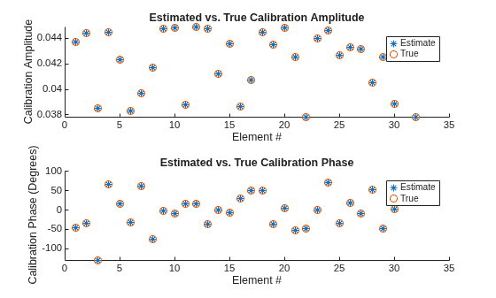
This method appears to work well with only $2N+1$ phase offset points, offering a faster alternative to REV.

Grouped REV Method

A major shortcoming of the previously described methods is that the change in power for a single element under test can become extremely small if the composite field vector is large, for example in an array with a large number of elements.

This issue can be alleviated by varying the phase of a group of elements simultaneously instead of calibrating a single element at a time [4].

In this approach a grouping matrix G is constructed where each row indicates the elements to be tested simultaneously. G typically takes the form:

$$G=\left[\begin{array}{ccccc}F& 0& 0& 0& 0\\ 0& F& 0& 0& 0\\ 0& 0& ...& 0& 0\\ 0& 0& 0& F& 0\\ 0& 0& 0& 0& F\end{array}\right]$$

Where $F$ is a $KxK$ basis matrix containing only 1s and 0s. $F$ doesn't technically need to be uniform throughout G, but it is here for simplicity.

For each row in the grouping matrix, one of the previously described power only calibration methods is performed, generating a composite calibration field vector $s$, which can be related to the individual element calibration values:

$$s=G\left(\frac{E_n}{E_0}\right)$$

As long as G can be inverted, we can solve for the individual element calibration values from $s$:

$$\frac{E_n}{E_0}=G^{-1}s$$

In the simplest case no grouping is performed and G is the identity matrix, in which case this method simplifies to the individual element approaches described in the previous sections.

There are different ways to construct the grouping matrix G, but it is important that the matrix be well-conditioned and the groups are large enough to be robust to noise. Refer to [4] for more information on robustly constructing G and also for some enhancements that can be made to this algorithm to improve performance beyond what is described in this example.

In the function below we provide a simple function for constructing the grouping matrix G.

function G = helperConstructG(numElements)
    % Construct the grouping matrix G, numElements must be a power of 2.
    
    % If the number of elements is less than some specified value, use the
    % identify matrix (i.e. test elements individually).
    minG = 8;
    if numElements < minG
        G = eye(numElements);
        return
    end

    % Get the size of the basis matrix
    basisSize = numElements/minG;

    % Construct G using Hadamard matrices for F
    G = ones(numElements)*-1;
    nBasis = numElements/basisSize;
    startIdx = 1;
    for iBasis = 1:nBasis
        endIdx = startIdx + basisSize-1;
        F = hadamard(basisSize);
        G(startIdx:endIdx,startIdx:endIdx) = F;
        startIdx = endIdx+1;
    end
    G = (G+1)/2;
end

Call this function for the number of elements in our test array and plot the output.

G = helperConstructG(numElements);
helperPlotGroupingMatrix(G);

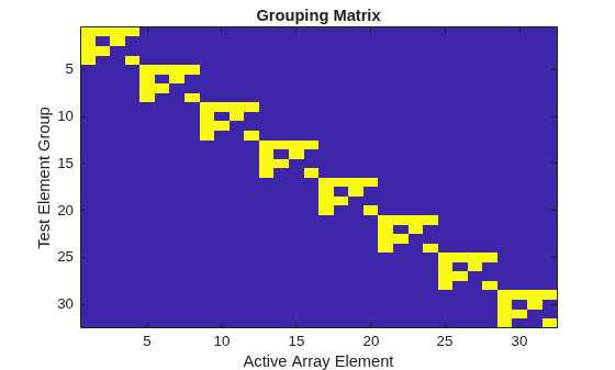
Each row in G describes a group of elements that are to be tested together. The yellow squares are active elements and the blue squares are inactive elements in each test group.

In the loop below, we use the best fit REV method on groups of elements indicated in G.

testPhaseShifts = helperGetEvenlySpacedPhases(8);
nPoints = length(testPhaseShifts);
groupCalWeights = ones(numElements,1);
for iElement = 1:numElements
    % Record the power measured for each group
    power = zeros(nPoints,1);

    % Get the group vector
    gv = logical(G(iElement,:))';

    % Measure power at each group phase shift
    for ips = 1:nPoints
        ps = testPhaseShifts(ips);
        testWeights = ones(numElements,1);
        testWeights(gv) = exp(1i*deg2rad(ps));
        power(ips) = helperMeasurePower(calSig,txAng,rxAng,radiator,collector,receiver,testWeights);
    end

    % Apply REV best fit algorithm to group.
    groupCalWeights(iElement) = helperRevBestFit(testPhaseShifts,power,1);
end

To get the final calibration weights, we solve the system of equations using G and the group calibration weights measured above.

% Calibration weights solved using group weights
estCalWeights = G\groupCalWeights;
helperShowCalibrationError(estCalWeights,trueCalWeights);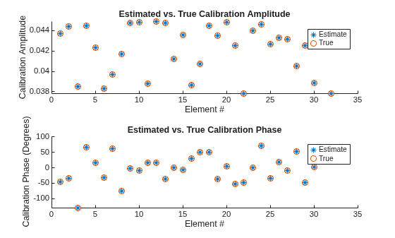

The grouped REV method also shows good calibration results. The benefit of this method will become apparent in a later section as the size of the array under test increases.

Ambiguity In Power Only Calibration

Ambiguity Demonstration

In both the REV and fast calibration method, there are two sets of equations that give the correct calibration values depending on whether $\left|{\underset{}{\overset{‾}{E}}}_n\right|>\left|E_n\right|$ or $\left|{\underset{}{\overset{‾}{E}}}_n\right|<\left|E_n\right|$. Oftentimes it is assumed that $\left|{\underset{}{\overset{‾}{E}}}_n\right|>\left|E_n\right|$, however depending on the nature of the array and the calibration errors, this may be a poor assumption.

In this section we demonstrate what happens if any of the elements being tested fall into the case where $\left|{\underset{}{\overset{‾}{E}}}_n\right|<\left|E_n\right|$.

First, set element 1 so that its magnitude is larger than the composite vector of the rest of the elements.

% Artificially introduce ambiguity into calibration errors
e1Bar = sum(calErr(2:end));
e1 = 2*abs(e1Bar)*exp(1i*angle(calErr(1)));
ambgCalErr = [e1 calErr(2:end)];

% Update array to contain the new calibration weights
release(radiator);
radiator.Sensor.Taper = ambgCalErr;

Measure the calibration power testing element 1 with the updated calibration weights.

% Record the power measured for each element
nPoints = 2^nBits;
revPhaseShifts = helperGetEvenlySpacedPhases(nPoints);
power = zeros(nPoints,1);

% Measure power at each phase shift
for ips = 1:nPoints
    ps = revPhaseShifts(ips);
    testWeights = ones(numElements,1);
    testWeights(1) = exp(1i*deg2rad(ps));
    power(ips) = helperMeasurePower(calSig,txAng,rxAng,radiator,collector,receiver,testWeights);
end

If we plot the measured power, it is still sinusoidal, the two cases are indistinguishable in general with only the provided power measurements.

helperDisplayPowerSinusoid(revPhaseShifts,power,1);

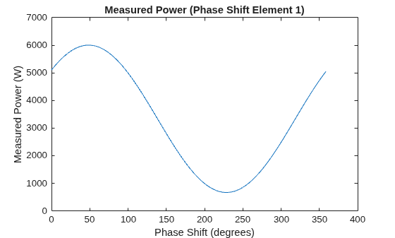
We can apply the case 1 equations and case 2 equations, and see that only case 2 give the correct values.

% Compare ambiguous cases
expCal1 = ambgCalErr(1)/sum(ambgCalErr);
cal1Case1 = helperRev(revPhaseShifts,power,1);
cal1Case2 = helperRev(revPhaseShifts,power,2);
helperCompareCalCases(expCal1,cal1Case1,cal1Case2,'REV Method');

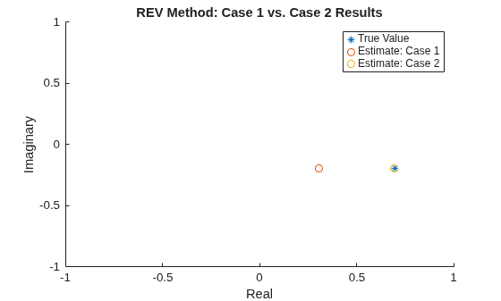
This ambiguity can result in incorrect calibration values in cases where $\left|{\underset{}{\overset{‾}{E}}}_n\right|<\left|E_n\right|$.

A similar demonstration can be shown for the fast calibration method.

% Record the power measured for each element
fastPhaseShifts = [0 90 180];
nPoints = length(fastPhaseShifts);
power = zeros(nPoints,1);

% Measure power at each phase shift
for ips = 1:nPoints
    ps = fastPhaseShifts(ips);
    testWeights = ones(numElements,1);
    testWeights(1) = exp(1i*deg2rad(ps));
    power(ips) = helperMeasurePower(calSig,txAng,rxAng,radiator,collector,receiver,testWeights);
end

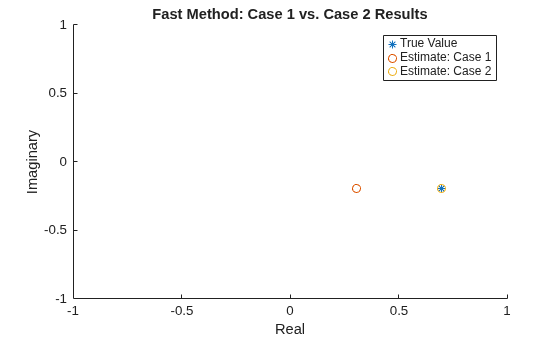
Comparing the results from the two sets of algorithms, we can see one gives incorrect values.

% Compare ambiguous cases
expCal1 = ambgCalErr(1)/sum(ambgCalErr);
cal1Case1 = helperFastCal(fastPhaseShifts,power,1);
cal1Case2 = helperFastCal(fastPhaseShifts,power,2);
helperCompareCalCases(expCal1,cal1Case1,cal1Case2,'Fast Method');

Resolving Ambiguity

There are a number of approaches that can be used to resolve this ambiguity in power only calibration, each of which requires some additional measurements. These approaches are discussed in [1] and [2].

One example of an approach that can be used and only requires a limited number additional measurements is described in more detail in [2]. The idea of this approach is to check whether ${\left|E\right|}_{\min }$ gets larger or smaller when the element under test is attenuated. If it gets larger, then $\left|{\underset{}{\overset{‾}{E}}}_n\right|>\left|E_n\right|$, and if it gets smaller then $\left|{\underset{}{\overset{‾}{E}}}_n\right|<\left|E_n\right|$. This resolution technique is demonstrated for REV.

% Record the power measured for element 1
eut = 1;
nPoints = 2^nBits;
revPhaseShifts = helperGetEvenlySpacedPhases(nPoints);
power = zeros(nPoints,1);

% Measure power at each phase shift
for ips = 1:nPoints
    ps = revPhaseShifts(ips);
    testWeights = ones(numElements,1);
    testWeights(eut) = exp(1i*deg2rad(ps));
    power(ips) = helperMeasurePower(calSig,txAng,rxAng,radiator,collector,receiver,testWeights);
end

% Get Emin magnitude and angle
[minPower,minPowerIdx] = min(power);
minPowerAng = revPhaseShifts(minPowerIdx);

% Take another measurement with reduced amplitude at the minimum shift
reducedAmp = 0.1;
reducedWeights = ones(numElements,1);
reducedWeights(eut) = reducedAmp*exp(1i*deg2rad(minPowerAng));
updatedMinPower = helperMeasurePower(calSig,txAng,rxAng,radiator,collector,receiver,reducedWeights);

% Determine the ambiguity based on the change in power
if updatedMinPower > minPower
    ambgCase = 1;
else
    ambgCase = 2;
end

% Show the case that was selected
disp(['Ambiguity Case: ',num2str(ambgCase)]);

Ambiguity Case: 2

% Get the calibration value based on the ambiguity case
measuredCal = helperRev(revPhaseShifts,power,ambgCase);

% Compare the true and estimated calibration value
trueCal = radiator.Sensor.Taper(eut)/sum(radiator.Sensor.Taper);
disp(['True Calibration Value: ',num2str(trueCal)]);

True Calibration Value: 0.69604-0.19571i

disp(['Estimated Calibration Value: ',num2str(measuredCal)]);

Estimated Calibration Value: 0.69518-0.19279i

Using this approach or similar approaches, it is possible to resolve the inherent ambiguity in power only calibration methods.

In the next section the calibration algorithms are compared across different measurement conditions. The calibration errors are constructed such that $\left|{\underset{}{\overset{‾}{E}}}_n\right|>\left|E_n\right|$. However, when developing a calibration scheme it may be necessary to clarify this ambiguity.

Calibration Algorithm Comparison

In this section we compare each of the power only calibration methods by simulating two measurement conditions to see which algorithms are fastest and most accurate by using a Monte Carlo approach. We parameterize the test across the following cases:

• Signal to noise ratio (SNR) of measurement setup - using a 32 element array, from 0 to 50 dB in 10 dB increments

• Number of array elements - SNR at 30 dB, from 4 to 64 elements (doubling each time)

The four algorithms compared are:

• Full REV: Classic REV exercising every phase available in the phase shifter.

• REV Sinusoidal Fit (8 points): REV using sinusoidal curve fitting with 8 measurement points per element.

• Fast Method: The fast calibration method using only 3 measurement points per element.

• Grouped REV using REV Sinusoidal Fit (8 points): REV performed by applying phase shifts to groups of elements instead of individual elements. Use 8 point curve fit on grouped elements.

For each test, we measure 30 sets of calibration weights. In order to measure the effectiveness of each calibration algorithm for each test case, we calculate the RMS error between the true calibration vector and the estimated calibration vector.

nRuns = 30;
algorithmNames = ["Full REV","REV Fit (8 pts)","Fast Method","Grouped REV"];
nAlgorithms = length(algorithmNames);

Sweep 1: Signal to Noise Ratio

In this sweep we fix the number of elements at 32 and phase deviation at 30 degrees, varying the measurement SNR from 0 dB up to 50 dB.

snrSweep = 0:10:50;
nSNRTests = length(snrSweep);
nElem = 32;
phaseDevDeg = 30;

% Create the array for this sweep
testArray = phased.ULA(NumElements=nElem,ElementSpacing=spacing);
testRadiator = phased.Radiator(Sensor=testArray,OperatingFrequency=fc,WeightsInputPort=true);

% Compute baseline signal power for SNR scaling
testSigPow = helperCollectedSignalPower(calSig,txAng,rxAng,ones(nElem,1),testRadiator,collector);
noisePow = 1/db2pow(awgnSnr);

rmsErrSNR = zeros(nSNRTests,nAlgorithms);

for iTest = 1:nSNRTests
    snrTarget = snrSweep(iTest);
    sigScale = sqrt(db2pow(snrTarget)*noisePow/testSigPow);

    rmsErrRuns = zeros(nRuns,nAlgorithms);

    for iRun = 1:nRuns
        % Generate random calibration errors ensuring case 1
        calErrRun = helperGenerateCalErrors(nElem,phaseDevDeg);

        % Set calibration errors on the array
        release(testRadiator);
        testRadiator.Sensor.Taper = calErrRun;

        % Scale calibration signal for desired SNR
        calSigScaled = calSig*sigScale;

        % True calibration weights
        trueWeights = calErrRun / sum(calErrRun);

        % Run each algorithm
        rmsErrRuns(iRun,:) = helperRunAllAlgorithms(nElem,calSigScaled,txAng,rxAng,testRadiator,collector,receiver,trueWeights);
    end

    rmsErrSNR(iTest,:) = mean(rmsErrRuns,1);
end

Plot the RMS calibration error as a function of SNR.

helperPlotComparisonSweep(snrSweep,rmsErrSNR, ...
    algorithmNames,'SNR (dB)','RMS Calibration Error', ...
    'Calibration Error vs. SNR');

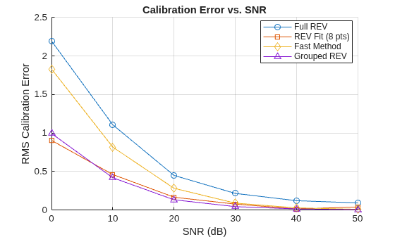
None of the algorithms work particularly well at low SNRs. This is typically not much of a concern because calibration happens in controlled environments where SNR is high. At high SNRs, the algorithms converge. It is interesting to point out that fitting a sinusoid to only 8 data points always performs better than collecting more data points but not performing this regression. This suggests that it may always be useful to perform this sinusoidal fit regardless of the number of data points collected during REV.

Sweep 2: Number of Array Elements

In this sweep we fix SNR at 30 dB and phase deviation at 30 degrees, varying the number of array elements from 4 to 64.

elementSweep = 4*2.^(0:4);
nElementTests = length(elementSweep);
snrTarget = 30;
phaseDevDeg = 30;

rmsErrElements = zeros(nElementTests,nAlgorithms);

for iTest = 1:nElementTests
    nElem = elementSweep(iTest);

    % Create a new array for this element count
    testArray = phased.ULA(NumElements=nElem,ElementSpacing=spacing);
    testRadiator = phased.Radiator(Sensor=testArray,OperatingFrequency=fc,WeightsInputPort=true);

    % Compute signal scaling for the desired SNR
    testSigPow = helperCollectedSignalPower(calSig,txAng,rxAng,ones(nElem,1),testRadiator,collector);
    noisePow = 1/db2pow(awgnSnr);
    sigScale = sqrt(db2pow(snrTarget)*noisePow/testSigPow);

    rmsErrRuns = zeros(nRuns,nAlgorithms);

    for iRun = 1:nRuns
        % Generate random calibration errors ensuring case 1
        calErrRun = helperGenerateCalErrors(nElem,phaseDevDeg);

        % Set calibration errors on the array
        release(testRadiator);
        testRadiator.Sensor.Taper = calErrRun;

        % Scale calibration signal for desired SNR
        calSigScaled = calSig*sigScale;

        % True calibration weights
        trueWeights = calErrRun / sum(calErrRun);

        % Run each algorithm
        rmsErrRuns(iRun,:) = helperRunAllAlgorithms(nElem,calSigScaled,txAng,rxAng,testRadiator,collector,receiver,trueWeights);
    end

    rmsErrElements(iTest,:) = mean(rmsErrRuns,1);
end

Plot the RMS calibration error as a function of array size.

helperPlotComparisonSweep(elementSweep,rmsErrElements, ...
    algorithmNames,'Number of Elements','RMS Calibration Error', ...
    'Calibration Error vs. Number of Elements');

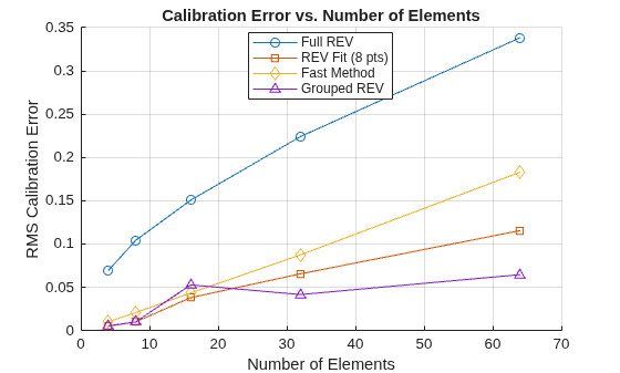
As the number of elements increase, the calibration accuracy degrades for each of the methods. However, the grouped REV method sees the least amount of degradation. For large arrays it may be necessary to group elements together so that the power variation is detectable.

Measurement Count Comparison

In addition to accuracy, the number of measurements required is a critical consideration when selecting a calibration algorithm. Fewer measurements means faster calibration time. The total number of measurements for each algorithm is:

• Full REV: $$N\times (2^B-1)+1$$ (where B is the number of phase shift bits)

• REV Sinusoidal Fit (8 points): $$7N+1$$

• Fast Method: $$2N+1$$

• Grouped REV (8 points): 7N+1

The following table shows the total measurement count for each algorithm at different array sizes.

nBitsForTable = 8;
measurementCounts = zeros(length(elementSweep),nAlgorithms);
for ii = 1:length(elementSweep)
    N = elementSweep(ii);
    measurementCounts(ii,1) = N*(2^nBitsForTable-1)+1;
    measurementCounts(ii,2) = 7*N+1;
    measurementCounts(ii,3) = 2*N+1;
    measurementCounts(ii,4) = 7*N+1;
end

measurementTable = array2table(measurementCounts, ...
    VariableNames=algorithmNames, ...
    RowNames=string(elementSweep)+" elements");
disp(measurementTable);

                   Full REV    REV Fit (8 pts)    Fast Method    Grouped REV
                   ________    _______________    ___________    ___________

    4 elements       1021             29                9             29    
    8 elements       2041             57               17             57    
    16 elements      4081            113               33            113    
    32 elements      8161            225               65            225    
    64 elements     16321            449              129            449    

Conclusion

In this example we investigated a few popular power only phased array calibration methods. We discussed their implementation and shortcomings such as potential issues with ambiguities in the calibration estimates. Finally, we compared these algorithms across array sizes, SNRs, and total number of measurements required.

References

[1] Mano et al. A Method for Measuring Amplitude and Phase of each Radiating Element of a Phased Array Antenna. Electronics and Communications in Japan (Part I: Communications). 1982.

[2] Yoon et al. Improved Rotating-Element Electric-Field Vector Method for Fast Far-Field Phased Array Calibration. IEEE Transactions on Antennas and Propagation. 2021.

[3] Long et al. Fast Amplitude-Only Measurement Method for Phased Array Calibration. IEEE Transactions on Antennas and Propagation. 2017.

[4] Fan et al. Large-Scale Phased Array Calibration Based on Amplitude-Only Measurement With the Multiround Grouped-REV Method. IEEE Transactions on Antennas and Propagation. 2024.

function power = helperMeasurePower(calSig,txAng,rxAng,radiator,collector,receiver,weights)
    % Simulate signal transmission and reception
    txSig = radiator(calSig,txAng,weights);
    collectSig = collector(txSig,rxAng);
    sigPower = receiver(collectSig);
    power = mean(sigPower);
end

function helperDisplayPowerSinusoid(testPhaseShifts,power,eut)
    ax = axes(figure);
    plot(ax,testPhaseShifts,power);
    xlabel(ax,'Phase Shift (degrees)');
    ylabel(ax,'Measured Power (W)');
    title(ax,['Measured Power (Phase Shift Element ',num2str(eut),')']);
end

function helperShowCalibrationError(estCalWeights,trueCalWeights)
    % Get estimated calibration amplitude and phase
    estAmp = abs(estCalWeights);
    estPhase = wrapTo180(rad2deg(angle(estCalWeights)));
    N = length(estCalWeights);

    % Get true calibration amplitude and phase
    trueAmp = abs(trueCalWeights);
    truePhase = wrapTo180(rad2deg(angle(trueCalWeights)));

    % Create a tiled layout
    f = figure;
    tl = tiledlayout(f,"vertical");
    
    % Plot amplitude
    ampAx = nexttile(tl);
    hold(ampAx,"on");
    title(ampAx,'Estimated vs. True Calibration Amplitude');
    xlabel(ampAx,'Element #')
    ylabel(ampAx,'Calibration Amplitude');
    scatter(ampAx,1:N,estAmp,'*',DisplayName='Estimate');
    scatter(ampAx,1:N,trueAmp,'o',DisplayName='True');
    legend(ampAx,Location="northeast");

    % Plot phase
    phaseAx = nexttile(tl);
    hold(phaseAx,"on");
    title(phaseAx,'Estimated vs. True Calibration Phase');
    xlabel(phaseAx,'Element #')
    ylabel(phaseAx,'Calibration Phase (Degrees)');
    scatter(phaseAx,1:N,estPhase,'*',DisplayName='Estimate');
    scatter(phaseAx,1:N,truePhase,'o',DisplayName='True');
    legend(phaseAx,Location="northeast");
end

function helperCompareCalCases(expected,case1,case2,methodName)
    % Compare results when using case 1 and case 2 equations for REV
    ax = axes(figure);
    hold(ax,"on");
    title(ax,[methodName,': Case 1 vs. Case 2 Results']);
    xlabel(ax,'Real');
    ylabel(ax,'Imaginary');
    scatter(ax,real(expected),imag(expected),'*',DisplayName='True Value');
    scatter(ax,real(case1),imag(case1),DisplayName='Estimate: Case 1');
    scatter(ax,real(case2),imag(case2),DisplayName='Estimate: Case 2');
    legend(ax);
    xlim(ax,[-1 1]);
    ylim(ax,[-1 1]);
end

function calErr = helperGenerateCalErrors(nElem,phaseDevDeg)
    % Generate random calibration errors ensuring that for every element,
    % the magnitude of the composite vector without that element is greater
    % than the magnitude of that element (case 1 ambiguity).
    valid = false;
    while ~valid
        ampErr = 1 + 0.2*rand(1,nElem);
        phaseErr = randn(1,nElem)*deg2rad(phaseDevDeg);
        calErr = ampErr.*exp(1i*phaseErr);

        % Check case 1 condition for all elements
        fullSum = sum(calErr);
        valid = true;
        for iElem = 1:nElem
            eBar = fullSum - calErr(iElem);
            if abs(eBar) <= abs(calErr(iElem))
                valid = false;
                break;
            end
        end
    end
end

function sigpow = helperCollectedSignalPower(calSig,txAng,rxAng,weights,radiator,collector)
    % Measure the received signal power at the output of the collector.
    txSig = radiator(calSig,txAng,weights);
    collectSig = collector(txSig,rxAng);
    sigpow = rms(collectSig)^2;
end

function rmsErr = helperRunAllAlgorithms(nElem,calSig,txAng,rxAng,radiator,collector,receiver,trueWeights)
    nAlgorithms = 4;
    estWeights = zeros(nAlgorithms,nElem);

    % Define phase shifts for each algorithm
    psFullRev = helperGetEvenlySpacedPhases(2^5);
    psFit8 = helperGetEvenlySpacedPhases(8);
    psFast = [0 90 180];

    % Full REV
    for iElem = 1:nElem
        power = helperMeasureElement(iElem,nElem,psFullRev,calSig,txAng,rxAng,radiator,collector,receiver);
        estWeights(1,iElem) = helperRev(psFullRev,power,1);
    end

    % REV sinusoidal fit (8 points)
    for iElem = 1:nElem
        power = helperMeasureElement(iElem,nElem,psFit8,calSig,txAng,rxAng,radiator,collector,receiver);
        estWeights(2,iElem) = helperRevBestFit(psFit8,power,1);
    end

    % Fast method
    for iElem = 1:nElem
        power = helperMeasureElement(iElem,nElem,psFast,calSig,txAng,rxAng,radiator,collector,receiver);
        estWeights(3,iElem) = helperFastCal(psFast,power,1);
    end

    % Grouped REV method
    nGroups = nElem;
    G = helperConstructG(nElem);
    groupCalWeights = zeros(nGroups,1);
    for iGroup = 1:nGroups
        groupIdx = logical(G(iGroup,:)');
        power = helperMeasureElementGroup(groupIdx,nElem,psFit8,calSig,txAng,rxAng,radiator,collector,receiver);
        groupCalWeights(iGroup) = helperRevBestFit(psFit8,power,1);
    end
    estWeights(4,:) = G\groupCalWeights;

    % Compute RMS error for each algorithm
    rmsErr = zeros(1,nAlgorithms);
    for iAlg = 1:nAlgorithms
        err = (estWeights(iAlg,:) - trueWeights)./abs(trueWeights);
        rmsErr(iAlg) = rms(err);
    end
end

function power = helperMeasureElement(iElem,nElem,phaseShifts,calSig,txAng,rxAng,radiator,collector,receiver)
    % Measure the power received by adding phase shifts to a single element
    nPoints = length(phaseShifts);
    power = zeros(nPoints,1);
    for ips = 1:nPoints
        testWeights = ones(nElem,1);
        testWeights(iElem) = exp(1i*deg2rad(phaseShifts(ips)));
        power(ips) = helperMeasurePower(calSig,txAng,rxAng,radiator,collector,receiver,testWeights);
    end
end

function power = helperMeasureElementGroup(groupIdx,nElem,phaseShifts,calSig,txAng,rxAng,radiator,collector,receiver)
    % Measure the power received by adding phase shifts to a group of
    % elements
    nPoints = length(phaseShifts);
    power = zeros(nPoints,1);
    for ips = 1:nPoints
        testWeights = ones(nElem,1);
        testWeights(groupIdx) = exp(1i*deg2rad(phaseShifts(ips)));
        power(ips) = helperMeasurePower(calSig,txAng,rxAng,radiator,collector,receiver,testWeights);
    end
end

function helperPlotComparisonSweep(xValues,rmsErr,algorithmNames,xLabel,yLabel,titleStr)
    % Plot algorithm comparisons
    f = figure;
    ax = axes(f);
    hold(ax,"on");
    markers = ['o','s','d','^'];
    for iAlg = 1:length(algorithmNames)
        plot(ax,xValues,rmsErr(:,iAlg), ...
            ['-',markers(iAlg)], ...
            DisplayName=algorithmNames(iAlg));
    end
    xlabel(ax,xLabel);
    ylabel(ax,yLabel);
    title(ax,titleStr);
    legend(ax,Location="best");
    grid(ax,"on");
end

function helperPlotGroupingMatrix(G)
    % Plot the grouping matrix from grouped REV
    ax = axes(figure);
    imagesc(ax,G);
    title(ax,'Grouping Matrix');
    ylabel(ax,'Test Element Group');
    xlabel(ax,'Active Array Element');
end

function ps = helperGetEvenlySpacedPhases(nPoints)
    % Get n evenly spaced points from 0 to 360 degrees without duplicates.
    allPs = linspace(0,360,nPoints+1);
    ps = allPs(1:end-1);
end