Sinc Antenna as Approximation for Array Response Pattern
This example shows how a sinc antenna element can approximate the radiation pattern of an array.
Create a 5-by-2 rectangular array of isotropic elements designed to work at an operating frequency of 3 GHz. Specify an element spacing equal to half the wavelength.
fc = 3e9;
lambda = freq2wavelen(fc);
array = phased.URA('ElementSpacing',lambda/2,'Size',[5 2]);
Compute the radiation pattern of the array. Specify a range of azimuth angles from –90° to 90° and zero elevation. Plot the unnormalized azimuth pattern in polar coordinates.
az = -90:0.5:90;

recopts = {'CoordinateSystem','rectangular','Type','powerdb'};
polopts = {'CoordinateSystem','polar','Type','powerdb'};

arrayPatternAz = pattern(array,fc,az,0,recopts{:});

pattern(array,fc,az,0,polopts{:})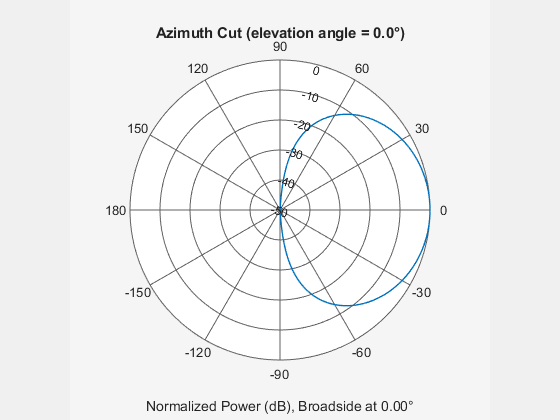
Normalize the pattern so that its maximum value is 0 dB. Compute the azimuth beamwidth.
arrayPatternAzNorm = arrayPatternAz - max(arrayPatternAz);
arrayAzBw = beamwidth(array,fc);
Compute the radiation for a range of elevation angles from –90° to 90° and zero azimuth. Normalize the pattern and compute the beamwidth. Plot the unnormalized elevation pattern in polar coordinates.
el = -90:0.5:90;

arrayPatternEl = pattern(array,fc,0,el,recopts{:});

arrayPatternElNorm = arrayPatternEl - max(arrayPatternEl);
arrayElBw = beamwidth(array,fc,'Cut','Elevation');

pattern(array,fc,0,el,polopts{:})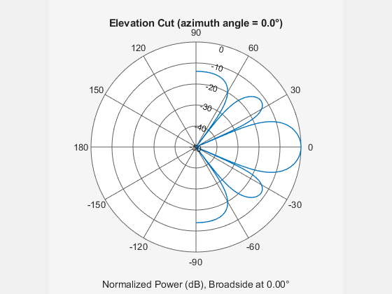
Create a sinc antenna element with the same beamwidth as the array. Compute the azimuth and elevation patterns. The patterns are normalized by construction.
se = phased.SincAntennaElement('Beamwidth',[arrayAzBw arrayElBw]);
sePatternAz = pattern(se,fc,az,0,recopts{:});
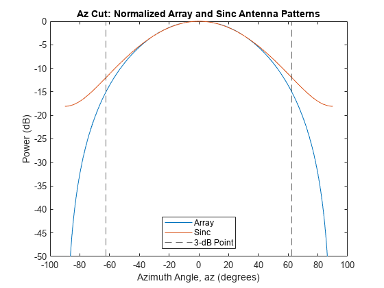
sePatternEl = pattern(se,fc,0,el,recopts{:});Find the smallest positive azimuth angle at which the patterns differ by about 3 dB. Plot the azimuth patterns in rectangular coordinates. Overlay the 3-dB points. The sinc azimuth pattern matches the array azimuth pattern well out to about 60 degrees.
idxAz = find((abs(arrayPatternAzNorm - sePatternAz) >= 3) & (az' >= 0),1);
az3dB = az(idxAz);

figure
plot(az,arrayPatternAzNorm,az,sePatternAz)
xline([-az3dB az3dB],'--')

title("Az Cut: Normalized Array and Sinc Antenna Patterns")
xlabel("Azimuth Angle, az (degrees)")
ylabel("Power (dB)")
legend("Array","Sinc","3-dB Point",Location="south")
ylim([-50 0])
Repeat the process for the elevation patterns. The sinc pattern is a good approximation out to about 20 degrees.
idxEl = find((abs(arrayPatternElNorm - sePatternEl) >= 3) & (el' >= 0),1);
el3dB = el(idxEl);

plot(el,arrayPatternElNorm,az,sePatternEl)
xline([-el3dB el3dB],'--')

title("El Cut: Normalized Array and Sinc Antenna Patterns")
xlabel("Elevation Angle, el (degrees)")
ylabel("Power (dB)")
legend("Array","Sinc","3-dB Point")
ylim([-50 0])
