Battery Second-Life Application State of Health (SoH) Estimation of Li-Ion Batteries
Traction batteries (such as EV batteries) have very specific energy and power requirements. The batteries must meet performance standards such as maintaining 80 percent of total usable capacity and a resting self-discharge rate of only about 5 percent over a 24-hour period. The batteries are subjected to extreme operating temperatures, large number of partial cycles, and changing discharge rates. These conditions cause significant battery degradation during the first few years of operation. To ensure safe operation, traction battery applications include expensive data collection and health monitoring systems which can compute capacity and state of health (SoH) accurately. When the battery can no longer meet these performance requirements, they are deemed to have reached End-of-Life status for the traction application.
However, a battery that has end-of-life status for the traction application can have a "second life" in less demanding applications such as smart grid (stationary) or low power electric vehicles such as golf carts. Second-life applications do not typically have access to an extensive measurement and monitoring infrastructure, but some level of monitoring is still necessary to prevent catastrophic failures.
This example shows an approach to monitoring second-life performance by estimating SoH using the measurements taken during first-life and only terminal voltage during second life. The approach uses a support vector regression (SVR) model to learn the relationship between extracted features and the discharge capacity of the battery during its first life. During its second life, the trained model is then used to estimate the SoH. For this example, SoH is defined to be energy focused and not for power delivery. When the SoH is low, the battery may not be able to provide enough charge for certain operations, and this may lead to application failure. Incorporating this SoH estimate can improve the accuracy of remaining useful life (RUL) predictions and provide more reliable estimation of a battery’s remaining capacity.
Data Set
NASA's battery aging data is used in this example. The data set contains measurements from commercially available Li-ion 18650 sized rechargeable batteries with rated capacity of 2 Ah at room temperature. The batteries are subjected to charge, constant current discharge, and electrochemical impedance spectroscopy cycles. These repeated charge and discharge cycles result in accelerated aging of the batteries while impedance measurements provide insight into the internal battery parameters that change as aging progresses. A total of 168 charging cycles are performed for battery cells B0005, B0006 and B0007. However, measurements for some cycles are incomplete, either because of incomplete measurement or repeated charging cycles without discharge. Measurements related to such incomplete cycles are removed before analysis. The data used in this example has been processed to contain only measurements related to normal cycles and those relevant to the features being extracted, such as, battery terminal voltage during charge/discharge of cycles. The original full data set with detailed description can be accessed here [2].
The data set contains measurements for three batteries titled B0005, B0006 and B0007. For this example, the data is assumed to represent batteries that are used for second life application. Measurements for the first 100 cycles is assumed to represent the first-life usage of the batteries. The remaining cycles are assumed to represent the measurements during their second-life application. Load the data from the MathWorks® support files site (about ~47 MB):
url = 'https://ssd.mathworks.com/supportfiles/predmaint/batteryagingdata/nasa/BatteryAgingData.zip';
websave('BatteryAgingData.zip',url);
unzip('BatteryAgingData.zip')
load('B0005.mat')
load('B0006.mat')
load('B0007.mat')
Extract the voltage measurements corresponding to charge, discharge cycle and capacity for each cycle for battery B0005 data set.
[B5_d, B5_c, C_B05] = hExtractChargeDischargeCycles(B0005);
To see the degradation of the battery's charge, discharge performance across cycles, plot the voltage over cycle numbers for charge cycle. The spread in the curves indicates that as the battery ages, the time taken to go from beginning of charge to 4.2 V increases. Similarly, the time taken for the battery to discharge decreases.
num_partial_cycles = 163;
figure; tiledlayout(2,1)
nexttile;
hold on
for i = 1:num_partial_cycles-1
plot(B5_c(i).t,B5_c(i).measuredV)
end
title('B0005 Voltage during Charging')
xlabel('Time [s]')
ylabel('Voltage')

nexttile
hold on;
for i = 1:num_partial_cycles-1
plot(B5_d(i).t,B5_d(i).measuredV)
end
title('B0005 Voltage during Discharging')
xlabel('Time [s]')
ylabel('Voltage')
![Figure contains 2 axes objects. Axes object 1 with title B0005 Voltage during Charging, xlabel Time [s], ylabel Voltage contains 162 objects of type line. Axes object 2 with title B0005 Voltage during Discharging, xlabel Time [s], ylabel Voltage contains 162 objects of type line.](../../examples/predmaint/win64/LiionBatterySecondLifeSoHExample_01.png)
Split the data into the first and second life related measurements using the hDataSplitter and hCapacitySplitter helper functions:
num_cycles_FirstLife = 100;
[B5_d_first, B5_c_first, B5_d_second, B5_c_second] = hDataSplitter(B5_d, B5_c, num_cycles_FirstLife);
[C_B05_first, C_B05_second] = hCapacitySplitter(C_B05, num_cycles_FirstLife);
Feature Extraction and State of Health
Measurement of maximum deliverable capacity for batteries in operation is difficult because the cells are not likely to be fully charged or discharged during operation. For such applications, two features that function as health indicators (HI) are computed with partial information are defined as:
Time Interval of an Equal Charging Voltage Difference (TIECVD) and
Time Interval of an Equal Discharging Voltage Difference (TIEDVD)
The selected features also fade with battery ageing, following the trend displayed by capacity fade. For charging voltage measurements, TIECVD is computed as the time interval taken to charge from 3.5 V to 4.2 V. For discharge voltage measurement, TIEDVD is computed as the time taken to discharge from 3.8 V and 3.6 V [1]. It is important to note that, for this data, the discharge is under constant current, which allows for TIEDVD to be a useful health indicator. If this is not the case, and discharge is based on a dynamic current profile instead, TIECVD alone must be used as a health indicator for SOH estimation, providing that the charge protocol is mostly fixed.
Compute the TIECVD/TIEDVD features for each battery using the helper function hFeatureExtraction. The helper function identifies the exact time instances, using interpolation, for each voltage value in the charge and discharge cycle and computes the features using the time stamps.
[TIECVD_B5_first, TIEDVD_B5_first] = hFeatureExtraction(B5_d_first, B5_c_first);
The definition of battery's SoH used in this example is:
where is the nominal capacity of the ith cycle and is the initial (rated) nominal capacity. The rated capacity of the cells in this data set is 2 Ah.
rated_C = 2;
SoH_B05_first = C_B05_first/rated_C;
Plot the computed features (TIECVD, TIEDVD) and the SoH of the batteries during their first life to visualize their trends.
figure;
nexttile;
title('Computed Features');
cyc_num = 1:num_cycles_FirstLife;
yyaxis left
plot(cyc_num,TIECVD_B5_first); hold on;
ylabel('TIECVD');
yyaxis right
plot(cyc_num,TIEDVD_B5_first, '-.');
ylabel('TIEDVD');
xlabel('Cycle Number')

nexttile
plot(cyc_num,SoH_B05_first);
ylabel('SoH')
xlabel('Cycle Number')

As seen in the plot, the curves of TIECVD/TIEDVD share similar characteristics with SoH with respect to the decreasing trend over cycle number. Given the similarity in trend and their ability to be computed online, these two HIs are suitable for battery health monitoring.
Model Development: Battery B0005
To develop and test the model, start by using only the measurements for battery B0005. Training data is defined to be the features computed for the first-life as predictors and SoH as response variable. Define predictors_first to be a 100x2 array with features and response_first to be the corresponding SoH values.
%% Partition of training data set
predictors_first = [TIECVD_B5_first, TIEDVD_B5_first];
response_first = SoH_B05_first;
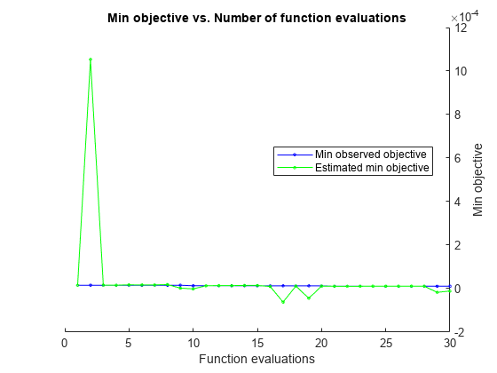
Support vector regression (SVR) model is considered to be a nonparametric model that works well for estimation, especially when the size of the training data set is limited. Fit an SVR model with a Gaussian kernel to build a nonlinear model for this regression problem and set the standardize option to be true to remove bias due to feature range differences. To further improve the fit, enable hyper parameter optimization as a part of the fit with five-fold cross validation and an iteration limit of 1000. Addtionally, vary the KernelFunction, NumGridDivisions, Kfold and IterationLimit to optimize the model training if required:
rng 'default'  % For reproducibility

sohEstimator = fitrsvm(predictors_first, response_first,...
    'KernelFunction', 'gaussian', ...
    'Standardize', true, ...
    'OptimizeHyperparameters', {'BoxConstraint','KernelScale','Epsilon'}, ...
    'HyperparameterOptimizationOptions', ...
    struct('AcquisitionFunctionName', 'expected-improvement-plus', ...
    'NumGridDivisions', 2,...
    'Repartition',true, ...
    'Kfold', 5), ...
    'IterationLimit', 1000,...
     'Verbose', 0)
|====================================================================================================================|
| Iter | Eval   | Objective:  | Objective   | BestSoFar   | BestSoFar   | BoxConstraint|  KernelScale |      Epsilon |
|      | result | log(1+loss) | runtime     | (observed)  | (estim.)    |              |              |              |
|====================================================================================================================|
|    1 | Best   |  1.5521e-05 |      2.8681 |  1.5521e-05 |  1.5521e-05 |        389.3 |       265.43 |    0.0028433 |
|    2 | Accept |   0.0040668 |     0.32302 |  1.5521e-05 |   0.0010533 |    0.0054226 |       442.27 |     0.011337 |
|    3 | Accept |   0.0037582 |     0.15809 |  1.5521e-05 |  1.5918e-05 |     0.067844 |       65.331 |       6.9157 |
|    4 | Accept |    0.003956 |     0.10668 |  1.5521e-05 |  1.5832e-05 |    0.0023879 |     0.028332 |    0.0052383 |
|    5 | Accept |  0.00010603 |     0.22419 |  1.5521e-05 |  1.7311e-05 |        996.4 |        17.83 |    0.0026153 |
|    6 | Accept |   0.0037452 |    0.047878 |  1.5521e-05 |  1.6835e-05 |       128.35 |     0.014707 |       3.5391 |
|    7 | Accept |    0.003084 |     0.04609 |  1.5521e-05 |  1.5594e-05 |       204.63 |     0.018262 |   0.00044168 |
|    8 | Accept |  1.5559e-05 |     0.06245 |  1.5521e-05 |  1.5066e-05 |       937.15 |       593.22 |   9.7286e-05 |
|    9 | Accept |   0.0036756 |    0.049572 |  1.5521e-05 |  1.5666e-05 |       933.04 |       359.05 |       6.5416 |
|   10 | Best   |  1.1395e-05 |    0.043165 |  1.1395e-05 | -5.6884e-05 |       955.34 |       184.19 |   0.00062026 |
|   11 | Accept |  1.2889e-05 |    0.043435 |  1.1395e-05 | -5.3534e-05 |       158.54 |       182.01 |   0.00028034 |
|   12 | Accept |  0.00012282 |    0.043361 |  1.1395e-05 | -3.5504e-05 |       236.16 |       974.67 |   0.00046029 |
|   13 | Best   |  1.0558e-05 |    0.055991 |  1.0558e-05 |  8.0133e-06 |       317.94 |       81.342 |    0.0011882 |
|   14 | Accept |  1.6142e-05 |    0.037953 |  1.0558e-05 |  6.7241e-06 |       224.12 |        304.4 |   8.5755e-05 |
|   15 | Accept |  1.1003e-05 |    0.044213 |  1.0558e-05 |  6.2727e-06 |       970.87 |       146.74 |   8.4215e-05 |
|   16 | Accept |  1.1324e-05 |    0.039446 |  1.0558e-05 |  4.8268e-06 |       992.93 |       83.217 |    0.0027571 |
|   17 | Accept |  1.2922e-05 |    0.044436 |  1.0558e-05 |  5.0712e-06 |       523.94 |          230 |   0.00018131 |
|   18 | Accept |  1.1325e-05 |    0.047344 |  1.0558e-05 | -8.2027e-07 |       461.83 |       132.73 |    0.0017491 |
|   19 | Accept |  1.3268e-05 |    0.044256 |  1.0558e-05 |   9.671e-07 |       155.91 |       57.106 |    8.561e-05 |
|   20 | Accept |  1.8032e-05 |    0.042428 |  1.0558e-05 |  1.6141e-06 |       967.26 |       637.41 |    0.0018164 |
|====================================================================================================================|
| Iter | Eval   | Objective:  | Objective   | BestSoFar   | BestSoFar   | BoxConstraint|  KernelScale |      Epsilon |
|      | result | log(1+loss) | runtime     | (observed)  | (estim.)    |              |              |              |
|====================================================================================================================|
|   21 | Best   |  1.0519e-05 |    0.049177 |  1.0519e-05 |  1.2575e-06 |       306.42 |        66.84 |   0.00019962 |
|   22 | Accept |  1.1093e-05 |    0.052478 |  1.0519e-05 |  3.0307e-06 |       996.76 |       153.63 |    0.0021315 |
|   23 | Accept |  1.2688e-05 |    0.047771 |  1.0519e-05 |  3.7094e-06 |       236.85 |       132.51 |   8.5046e-05 |
|   24 | Accept |  1.1488e-05 |    0.043183 |  1.0519e-05 |  4.7703e-06 |       62.184 |        58.49 |   0.00026719 |
|   25 | Accept |  1.1317e-05 |    0.047295 |  1.0519e-05 |  3.8174e-06 |       100.13 |       29.285 |    0.0040076 |
|   26 | Accept |   1.248e-05 |     0.04833 |  1.0519e-05 |  2.1295e-06 |       128.85 |       41.857 |     0.001427 |
|   27 | Accept |  1.1561e-05 |    0.045405 |  1.0519e-05 |   2.204e-06 |       201.55 |       55.888 |    0.0039601 |
|   28 | Accept |  1.1492e-05 |    0.038702 |  1.0519e-05 |  4.1126e-06 |       154.38 |       86.584 |   0.00022099 |
|   29 | Accept |  1.3752e-05 |    0.041626 |  1.0519e-05 |  4.3913e-06 |       57.581 |       84.719 |   8.5604e-05 |
|   30 | Accept |  1.1311e-05 |    0.040888 |  1.0519e-05 |  4.5135e-06 |       260.76 |        57.95 |    0.0027841 |

__________________________________________________________
Optimization completed.
MaxObjectiveEvaluations of 30 reached.
Total function evaluations: 30
Total elapsed time: 19.5825 seconds
Total objective function evaluation time: 4.827

Best observed feasible point:
    BoxConstraint    KernelScale     Epsilon
    _____________    ___________    __________

       306.42           66.84       0.00019962

Observed objective function value = 1.0519e-05
Estimated objective function value = 1.6276e-05
Function evaluation time = 0.049177

Best estimated feasible point (according to models):
    BoxConstraint    KernelScale     Epsilon
    _____________    ___________    __________

       154.38          86.584       0.00022099

Estimated objective function value = 4.5135e-06
Estimated function evaluation time = 0.054473
sohEstimator =
  RegressionSVM
                         ResponseName: 'Y'
                CategoricalPredictors: []
                    ResponseTransform: 'none'
                                Alpha: [91×1 double]
                                 Bias: 0.1045
                     KernelParameters: [1×1 struct]
                                   Mu: [2.7856e+03 788.3715]
                                Sigma: [393.9771 112.4298]
                      NumObservations: 100
    HyperparameterOptimizationResults: [1×1 classreg.learning.paramoptim.SupervisedLearningBayesianOptimization]
                       BoxConstraints: [100×1 double]
                      ConvergenceInfo: [1×1 struct]
                      IsSupportVector: [100×1 logical]
                               Solver: 'SMO'


  Properties, Methods
After fitting the model on data from the first life, validate the model performance for second life.
[TIECVD_B5_second, TIEDVD_B5_second] = hFeatureExtraction(B5_d_second, B5_c_second);

predictors_second = [TIECVD_B5_second, TIEDVD_B5_second];
SoH_B05_second = C_B05_second/rated_C;
cycles_second = num_cycles_FirstLife+1:numel(C_B05);

% Store the predicted signal
SoH_B05_second_estimate = predict(sohEstimator,predictors_second);
Performance Evaluation of Trained Model
To evaluate the result, predict and compute the RMSE of the estimated SoH.
RMSE_B05 = rmse(SoH_B05_second, SoH_B05_second_estimate);
Visualize the predicted vs. actual cycle life plot for the test data.
plot(cycles_second, SoH_B05_second)
hold on
plot(cycles_second, SoH_B05_second_estimate)
legend('Actual','Estimated')
title('SoH Estimation Plot')
xlabel('Cycle Number')
ylabel('SoH')
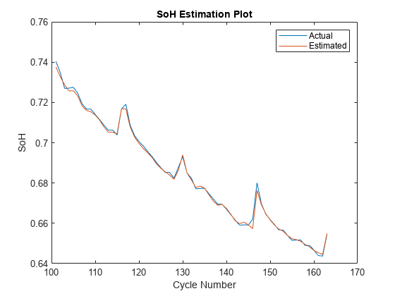
The plot indicates that SoH during the second life application of the cell can be estimated with reasonable accuracy by using the TIECVD/TIEDVD features and the SVR model trained on measurements from the first life application. Apply this approach to the data measured from batteries B0006 and B0007 to estimate its robustness.
Data Sets B0006 and B0007
Use the hTrainandEstimateSoH helper function to estimate the SoH for the second life application of batteries B0006 and B0007. The helper function implements the algorithm used above to:
Split the data into the first 100 cycles corresponding to the first life application
Compute first life features and SoH
Train SVR model
Compute second life features
Use the trained SVR model to estimate SoH for second life
[SoH_B06_second_estimate, SoH_B06_second] = hTrainandEstimateSoH(B0006, rated_C, num_cycles_FirstLife);
|====================================================================================================================|
| Iter | Eval   | Objective:  | Objective   | BestSoFar   | BestSoFar   | BoxConstraint|  KernelScale |      Epsilon |
|      | result | log(1+loss) | runtime     | (observed)  | (estim.)    |              |              |              |
|====================================================================================================================|
|    1 | Best   |  0.00024122 |     0.15676 |  0.00024122 |  0.00024122 |        389.3 |       265.43 |    0.0046115 |
|    2 | Accept |   0.0097686 |    0.056434 |  0.00024122 |   0.0007434 |    0.0054226 |       442.27 |     0.018387 |
|    3 | Accept |   0.0095499 |    0.048935 |  0.00024122 |  0.00024217 |     0.067844 |       65.331 |       11.217 |
|    4 | Accept |   0.0092904 |    0.058161 |  0.00024122 |  0.00024195 |    0.0023879 |     0.028332 |    0.0084959 |
|    5 | Accept |  0.00029944 |    0.051856 |  0.00024122 |  0.00024454 |        996.4 |       15.544 |    0.0042417 |
|    6 | Accept |  0.00058054 |    0.061319 |  0.00024122 |  0.00024999 |       543.03 |       139.36 |     0.031635 |
|    7 | Accept |  0.00034431 |    0.046349 |  0.00024122 |  0.00035984 |       506.75 |       23.621 |   0.00013659 |
|    8 | Accept |   0.0093514 |    0.044205 |  0.00024122 |  0.00024219 |       998.95 |       788.01 |       1.1818 |
|    9 | Accept |   0.0047676 |    0.044283 |  0.00024122 |  0.00024178 |       9.1108 |       293.17 |   0.00014355 |
|   10 | Accept |  0.00026804 |    0.046702 |  0.00024122 |  0.00024153 |       979.97 |       762.36 |   0.00045478 |
|   11 | Best   |  0.00023521 |    0.050209 |  0.00023521 |  0.00022818 |       471.07 |       31.317 |     0.011866 |
|   12 | Accept |   0.0015531 |    0.046791 |  0.00023521 |  0.00023308 |       918.07 |     0.061329 |   0.00014321 |
|   13 | Accept |  0.00027319 |    0.051403 |  0.00023521 |  0.00023221 |       273.51 |       777.52 |   0.00034256 |
|   14 | Accept |  0.00025431 |    0.045471 |  0.00023521 |  0.00023156 |       701.21 |       697.99 |    0.0087582 |
|   15 | Accept |  0.00024907 |    0.054468 |  0.00023521 |  0.00023135 |       415.99 |       702.62 |   0.00014247 |
|   16 | Accept |  0.00025128 |    0.050389 |  0.00023521 |  0.00023059 |       466.26 |       30.954 |    0.0008969 |
|   17 | Accept |  0.00030498 |    0.051341 |  0.00023521 |   0.0002281 |       629.38 |       935.07 |    0.0013602 |
|   18 | Accept |  0.00024129 |     0.04552 |  0.00023521 |  0.00020813 |       486.37 |       190.34 |   0.00027523 |
|   19 | Accept |   0.0095526 |    0.047378 |  0.00023521 |  0.00022923 |       132.04 |    0.0010393 |    0.0087388 |
|   20 | Best   |  0.00023328 |    0.039326 |  0.00023328 |  0.00022669 |       961.62 |       153.83 |    0.0068647 |
|====================================================================================================================|
| Iter | Eval   | Objective:  | Objective   | BestSoFar   | BestSoFar   | BoxConstraint|  KernelScale |      Epsilon |
|      | result | log(1+loss) | runtime     | (observed)  | (estim.)    |              |              |              |
|====================================================================================================================|
|   21 | Accept |  0.00075556 |    0.056661 |  0.00023328 |  0.00022618 |       980.06 |       15.878 |   0.00016777 |
|   22 | Accept |  0.00042116 |    0.042828 |  0.00023328 |   0.0002254 |       182.02 |       9.0994 |   0.00015237 |
|   23 | Accept |  0.00026872 |    0.041899 |  0.00023328 |  0.00022458 |       457.65 |          116 |     0.010767 |
|   24 | Accept |  0.00026231 |    0.046719 |  0.00023328 |  0.00023118 |       843.07 |       60.494 |     0.014257 |
|   25 | Best   |  0.00018434 |    0.047941 |  0.00018434 |  0.00018275 |       502.41 |       40.544 |    0.0043725 |
|   26 | Accept |  0.00028226 |    0.048144 |  0.00018434 |  0.00018142 |       227.81 |       38.695 |    0.0013518 |
|   27 | Accept |  0.00024837 |    0.044832 |  0.00018434 |  0.00018328 |       543.11 |       725.02 |   0.00031435 |
|   28 | Accept |  0.00025543 |    0.043756 |  0.00018434 |  0.00018282 |       282.66 |       86.615 |   0.00016358 |
|   29 | Accept |   0.0094348 |    0.035765 |  0.00018434 |  0.00018257 |    0.0010204 |    0.0024425 |       12.996 |
|   30 | Accept |  0.00022861 |    0.047214 |  0.00018434 |  0.00019051 |       476.02 |       63.603 |    0.0026303 |

__________________________________________________________
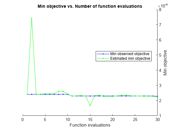
Optimization completed.
MaxObjectiveEvaluations of 30 reached.
Total function evaluations: 30
Total elapsed time: 9.1095 seconds
Total objective function evaluation time: 1.5531

Best observed feasible point:
    BoxConstraint    KernelScale     Epsilon
    _____________    ___________    _________

       502.41          40.544       0.0043725

Observed objective function value = 0.00018434
Estimated objective function value = 0.00019051
Function evaluation time = 0.047941

Best estimated feasible point (according to models):
    BoxConstraint    KernelScale     Epsilon
    _____________    ___________    _________

       502.41          40.544       0.0043725

Estimated objective function value = 0.00019051
Estimated function evaluation time = 0.049765
[SoH_B07_second_estimate, SoH_B07_second] = hTrainandEstimateSoH(B0007, rated_C, num_cycles_FirstLife);
|====================================================================================================================|
| Iter | Eval   | Objective:  | Objective   | BestSoFar   | BestSoFar   | BoxConstraint|  KernelScale |      Epsilon |
|      | result | log(1+loss) | runtime     | (observed)  | (estim.)    |              |              |              |
|====================================================================================================================|
|    1 | Best   |  2.4624e-05 |    0.039122 |  2.4624e-05 |  2.4624e-05 |        389.3 |       265.43 |    0.0027997 |
|    2 | Accept |   0.0032604 |    0.047764 |  2.4624e-05 |   0.0014541 |    0.0054226 |       442.27 |     0.011163 |
|    3 | Accept |   0.0030991 |    0.055051 |  2.4624e-05 |  2.4944e-05 |     0.067844 |       65.331 |       6.8095 |
|    4 | Accept |   0.0029705 |    0.052166 |  2.4624e-05 |  2.4829e-05 |    0.0023879 |     0.028332 |    0.0051578 |
|    5 | Accept |  8.2897e-05 |    0.063521 |  2.4624e-05 |  2.5279e-05 |        996.4 |       15.544 |    0.0019113 |
|    6 | Accept |     0.00308 |    0.037506 |  2.4624e-05 |  2.5342e-05 |       258.09 |     0.001074 |       3.5377 |
|    7 | Accept |   9.192e-05 |    0.045202 |  2.4624e-05 |  2.5498e-05 |       97.954 |      0.12088 |   0.00064409 |
|    8 | Accept |  4.6564e-05 |    0.042825 |  2.4624e-05 |  2.6342e-05 |          821 |       32.761 |   8.4169e-05 |
|    9 | Accept |  2.6277e-05 |    0.049264 |  2.4624e-05 |   2.555e-05 |       409.41 |       453.78 |    0.0005217 |
|   10 | Accept |  4.9061e-05 |    0.058545 |  2.4624e-05 |   2.607e-05 |       103.97 |       11.984 |   8.2586e-05 |
|   11 | Accept |  0.00020079 |    0.043554 |  2.4624e-05 |  2.0059e-05 |       290.92 |      0.13417 |   0.00013761 |
|   12 | Accept |  2.9871e-05 |    0.052707 |  2.4624e-05 |  2.6011e-05 |       3.0309 |       83.754 |   8.5293e-05 |
|   13 | Accept |   0.0023245 |     0.04394 |  2.4624e-05 |  0.00019861 |       27.278 |       955.63 |   0.00035476 |
|   14 | Accept |   0.0030515 |    0.039005 |  2.4624e-05 |  2.4033e-05 |       948.96 |    0.0011719 |    8.527e-05 |
|   15 | Accept |   0.0030243 |    0.051192 |  2.4624e-05 | -5.3995e-05 |       5.0054 |       1.5708 |       0.8005 |
|   16 | Accept |  0.00027292 |    0.041711 |  2.4624e-05 |  2.4166e-05 |       121.18 |       3.4117 |   0.00022876 |
|   17 | Accept |  4.7873e-05 |    0.037755 |  2.4624e-05 |  2.4199e-05 |       295.58 |       15.798 |    0.0092973 |
|   18 | Accept |    0.003016 |     0.04492 |  2.4624e-05 |  2.4583e-05 |       974.37 |        329.5 |       4.1635 |
|   19 | Accept |  3.4834e-05 |    0.039336 |  2.4624e-05 |  2.8499e-06 |        164.5 |       78.651 |   0.00045525 |
|   20 | Accept |  0.00019837 |    0.040317 |  2.4624e-05 |  2.4759e-05 |       384.37 |        12.97 |    0.0003702 |
|====================================================================================================================|
| Iter | Eval   | Objective:  | Objective   | BestSoFar   | BestSoFar   | BoxConstraint|  KernelScale |      Epsilon |
|      | result | log(1+loss) | runtime     | (observed)  | (estim.)    |              |              |              |
|====================================================================================================================|
|   21 | Accept |   5.343e-05 |    0.052263 |  2.4624e-05 |  2.4767e-05 |       4.6152 |       7.5921 |   8.5288e-05 |
|   22 | Accept |  3.2409e-05 |    0.048129 |  2.4624e-05 |   2.496e-05 |       874.12 |       146.43 |   0.00095241 |
|   23 | Accept |  3.3888e-05 |    0.042661 |  2.4624e-05 |    2.47e-05 |       533.26 |       266.35 |   0.00014048 |
|   24 | Accept |  4.3736e-05 |    0.036625 |  2.4624e-05 |  2.4775e-05 |      0.73009 |       23.577 |   8.5992e-05 |
|   25 | Accept |  3.9919e-05 |    0.041676 |  2.4624e-05 |  2.4735e-05 |       26.532 |      0.27039 |   9.2431e-05 |
|   26 | Accept |    2.73e-05 |    0.037949 |  2.4624e-05 |  2.4515e-05 |       1.6996 |       21.505 |   8.9624e-05 |
|   27 | Accept |   6.769e-05 |    0.047052 |  2.4624e-05 |  2.4501e-05 |       875.92 |      0.28924 |    0.0011327 |
|   28 | Accept |  3.6444e-05 |    0.040628 |  2.4624e-05 |  2.4518e-05 |      0.03828 |       1.0191 |   8.5245e-05 |
|   29 | Accept |  9.5558e-05 |      0.0438 |  2.4624e-05 |  2.4521e-05 |       39.363 |      0.82266 |   8.8101e-05 |
|   30 | Accept |  3.8507e-05 |    0.039468 |  2.4624e-05 |  2.4507e-05 |      0.34735 |      0.38742 |   0.00071323 |

__________________________________________________________
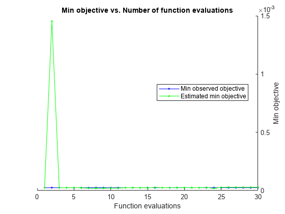
Optimization completed.
MaxObjectiveEvaluations of 30 reached.
Total function evaluations: 30
Total elapsed time: 7.6252 seconds
Total objective function evaluation time: 1.3557

Best observed feasible point:
    BoxConstraint    KernelScale     Epsilon
    _____________    ___________    _________

        389.3          265.43       0.0027997

Observed objective function value = 2.4624e-05
Estimated objective function value = 2.4507e-05
Function evaluation time = 0.039122

Best estimated feasible point (according to models):
    BoxConstraint    KernelScale     Epsilon
    _____________    ___________    _________

        389.3          265.43       0.0027997

Estimated objective function value = 2.4507e-05
Estimated function evaluation time = 0.044738
Performance Evaluation of Trained Model
Plot the predicted vs. actual SoH plot from validation data. The SoH data was predicted using the model trained from the first 100 cycles from data set.
Next, compute the SoH estimation RMSE for each battery to qualify the robustness of the approach.
figure;
subplot(3,1,1);
plot(SoH_B05_second)
hold on
plot(SoH_B05_second_estimate)
legend('Actual','Estimated');
title('SoH Estimation Plot for B0005')
xlabel('Cycle Number')
ylabel('SoH')

subplot(3,1,2);
plot(SoH_B06_second)
hold on
plot(SoH_B06_second_estimate)
legend('Actual','Estimated');
title('SoH Estimation Plot for B0006')
xlabel('Cycle Number')
ylabel('SoH')

subplot(3,1,3);
plot(SoH_B07_second)
hold on
plot(SoH_B07_second_estimate)
legend('Actual','Estimated');
title('SoH Estimation Plot for B0007')
xlabel('Cycle Number')
ylabel('SoH')
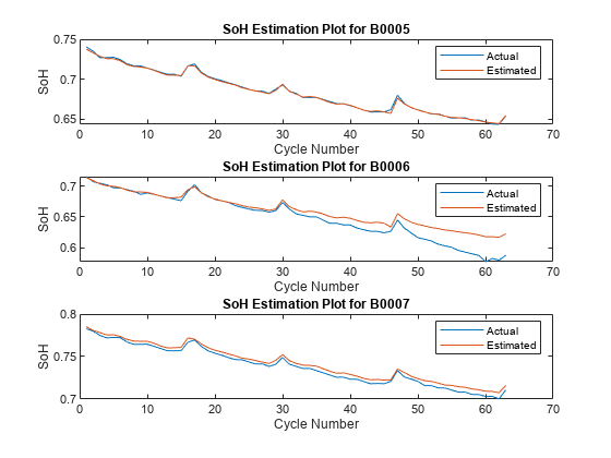
Compute the SOH estimation RMSE for each battery to qualify the robustness of the approach.
RMSE_B06 = rmse(SoH_B06_second, SoH_B06_second_estimate)
RMSE_B06 =
0.0337
RMSE_B07 = rmse(SoH_B07_second, SoH_B07_second_estimate)
RMSE_B07 =
0.0051
Conclusion
This example illustrates the estimation of Li-ion battery State of Health estimation for second-life applications. The estimation is based on two health indicators (HI), TIEDVD and TIECVD and an SVR model trained with first-life data. The selected HIs share a similar characteristic with battery capacity degradation over cycle number. Further, the HIs can be computed online thereby enabling online SoH estimation with relatively low complexity. This approach was robust across different batteries because the model was trained individually on each battery’s first-life measurements:
BattName = {'B0005';'B0006';'B0007'};
RMSE = [RMSE_B05;RMSE_B06;RMSE_B07];
table(string(BattName), RMSE, 'VariableNames', {'BattName', 'RMSE'})ans=3×2 table
"B0005" 0.0083
"B0006" 0.0337
"B0007" 0.0051
Temperature is also assumed to be constant across cycles in this example. However, temperature would vary from cycle to cycle during charge and this will impact the selected health indicators. To address this, temperature as an additional predictor can be explored.
Supporting Functions
function [SoH_estimate, SoH_second] = hTrainandEstimateSoH(Batt_data, rated_C, num_cycles_FirstLife)
% HTRAINANDESTIMATESOH function accepts battery measurements in the form of
% a structure, rated capacity to compute SoH, and number of cycles related
% to first life usage of the cell. The two health indicators TIECVD, and TIEDVD are computed and an
% support vector regression model is trained to estimate the SoH.

% Use the hExtractChargeDischargeCycles helper function to extract charge
% and discharge segments, and discharge capacity for each cycle.
[B_d, B_c, C_B] = hExtractChargeDischargeCycles(Batt_data);

% Call hDataSplitter helper function to split the charge and discharge data
% between the first and second life measurements
[B_d_first, B_c_first, B_d_second, B_c_second] = hDataSplitter(B_d, B_c, num_cycles_FirstLife);

% Split capacity measurements as well
[C_first, C_second] = hCapacitySplitter(C_B, num_cycles_FirstLife);

% Call hFeatureExtraction helper function to compute TIECVD and TIEDVD
[TIECVD_first, TIEDVD_first] = hFeatureExtraction(B_d_first, B_c_first);

% Compute SoH for first and second lives
SoH_first = C_first/rated_C;
SoH_second = C_second/rated_C;

[TIECVD_second, TIEDVD_second] = hFeatureExtraction(B_d_second, B_c_second);
predictors_second = [TIECVD_second, TIEDVD_second];

% Set up predictors and response to train the SVR model using first life
% measurements
predictors = [TIECVD_first, TIEDVD_first];
response = SoH_first;


%% SVR training
rng 'default'  % For reproducibility

regressionSVM = fitrsvm(predictors, response,...
    'KernelFunction', 'gaussian', ...
    'Standardize', true, ...
    'OptimizeHyperparameters', {'BoxConstraint','KernelScale','Epsilon'}, ...
    'HyperparameterOptimizationOptions', ...
    struct('AcquisitionFunctionName', 'expected-improvement-plus', ...
    'NumGridDivisions', 2,...
    'Repartition',true, ...
    'Kfold', 5), ...
    'IterationLimit', 1000,...
     'Verbose', 0);

% Estimate SoH for second life measurements
SoH_estimate = predict(regressionSVM,predictors_second);

end

function [B_d_first, B_c_first, B_d_second, B_c_second] = hDataSplitter(B_d, B_c, num_cycles_FirstLife)
% Function to split charge and discharge voltage measurements vector into
% two segments using the num_cycles_FirstLife value
    B_d_first  = B_d(1:num_cycles_FirstLife);
    B_c_first  = B_c(1:num_cycles_FirstLife);
    B_d_second = B_d(num_cycles_FirstLife+1:end);
    B_c_second = B_c(num_cycles_FirstLife+1:end);
end

function [C_first, C_second] = hCapacitySplitter(C, num_cycles_FirstLife)
% Function to split capacity measurements into two segments using the
% num_cycles_FirstLife value
    C_first = C(1:num_cycles_FirstLife);
    C_second = C(num_cycles_FirstLife+1:end);
end
References
[1] Zhao, Qi, Xiaoli Qin, Hongbo Zhao, and Wenquan Feng. “A Novel Prediction Method Based on the Support Vector Regression for the Remaining Useful Life of Lithium-Ion Batteries.” Microelectronics Reliability, vol. 85, June 2018, pp. 99–108. DOI.org (Crossref), https://doi.org/10.1016/j.microrel.2018.04.007.